
BatchDrake
Hacking, HAM Radio (EA1IYR), DSP, physics and more
Hacking, HAM Radio (EA1IYR), DSP, physics and more
(This post is a continuation of CTS @ HardWear.io 2020 - Write-up (I))
According to the previous challenge’s flag, frequency was 514 MHz and syncword 0x4F. The description of the challenge was as follows:
I guess you’re really into RF hacking if you’ve gotten this far!
I don’t need to tell you what to do to get to the next signal ;-)
Once you decoded that, enter the flag here!
Tuning to the referred signal produced a 192 ksps sample stream, with a train of bursty signals:
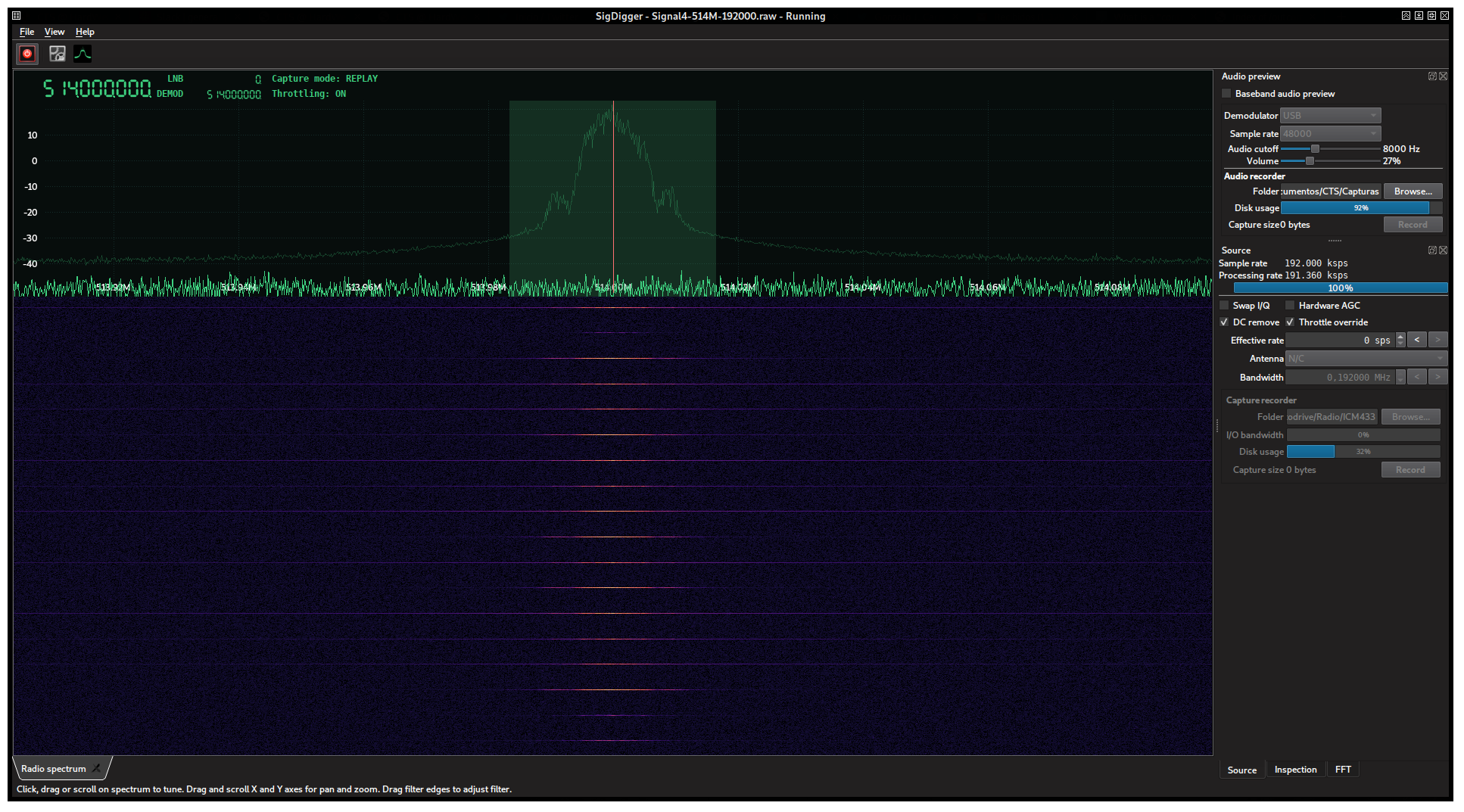
Since these bursts are again too short, their time inspection make sense. We can do it either by pressing the “Hold” button until they show up or by holding “Autosequelch” for a brief period of time (enough to measure the noise floor). Posterior analysis revealed that all bursts were basically the same burst repeated again and again, so it should be enough to isolate just one.
By analyzing the signal in the spectrogram, we can tell that although most of the energy (and probably the information) is concentrated in a main lobe roughly 24 kHz wide, it is not perfectly band-limited: there’s a some noticeable energy spread around the burst, decreasing with the distance to the central frequency. This out-of-band energy, which is actually redundant with respect to the true information contained in the burst, is called the skirt and it is caused by the pulse shaping function not being band-limited.
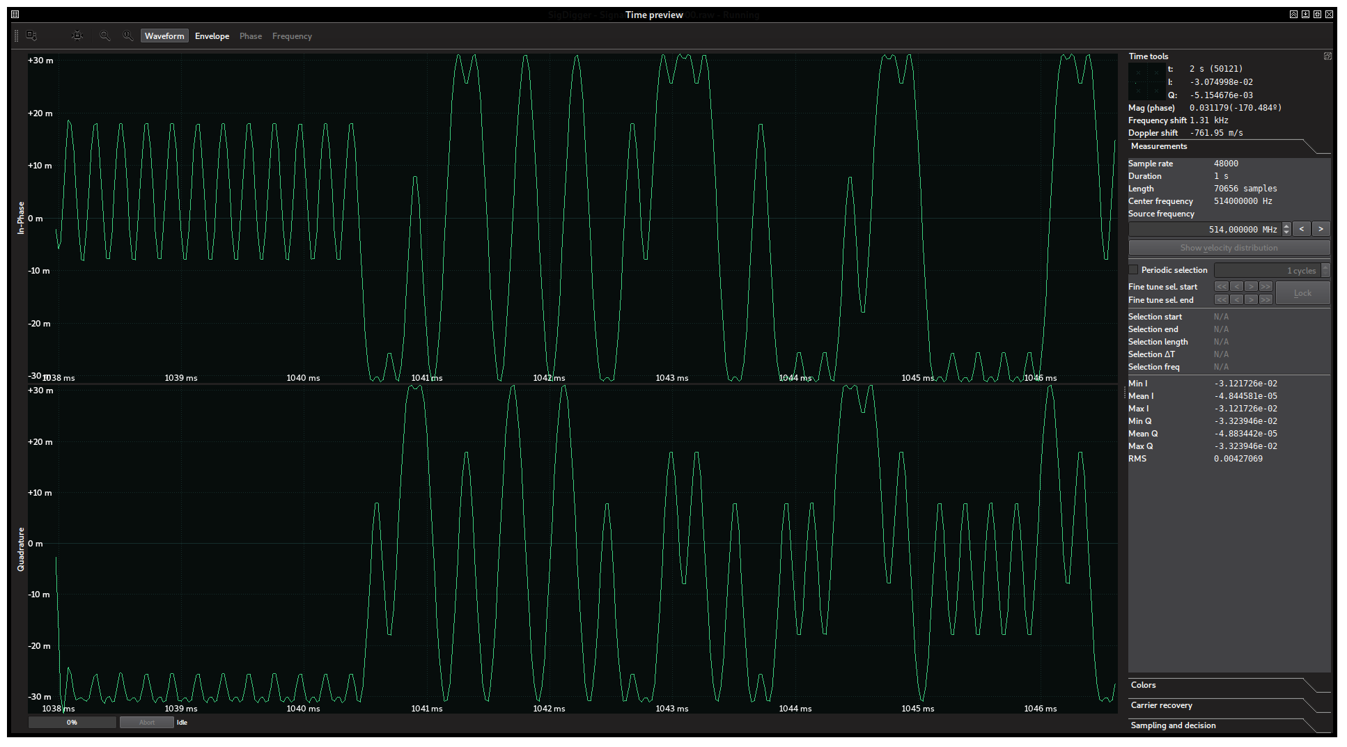
By clicking “Envelope”, a shape fitting the instantaneous amplitude of the signal is drawn behind its waveform. Its rectangular shape lets us conclude that we are dealing with a constant-envelope signal and therefore cannot be amplitude modulated (like the signal in the previous challenge).
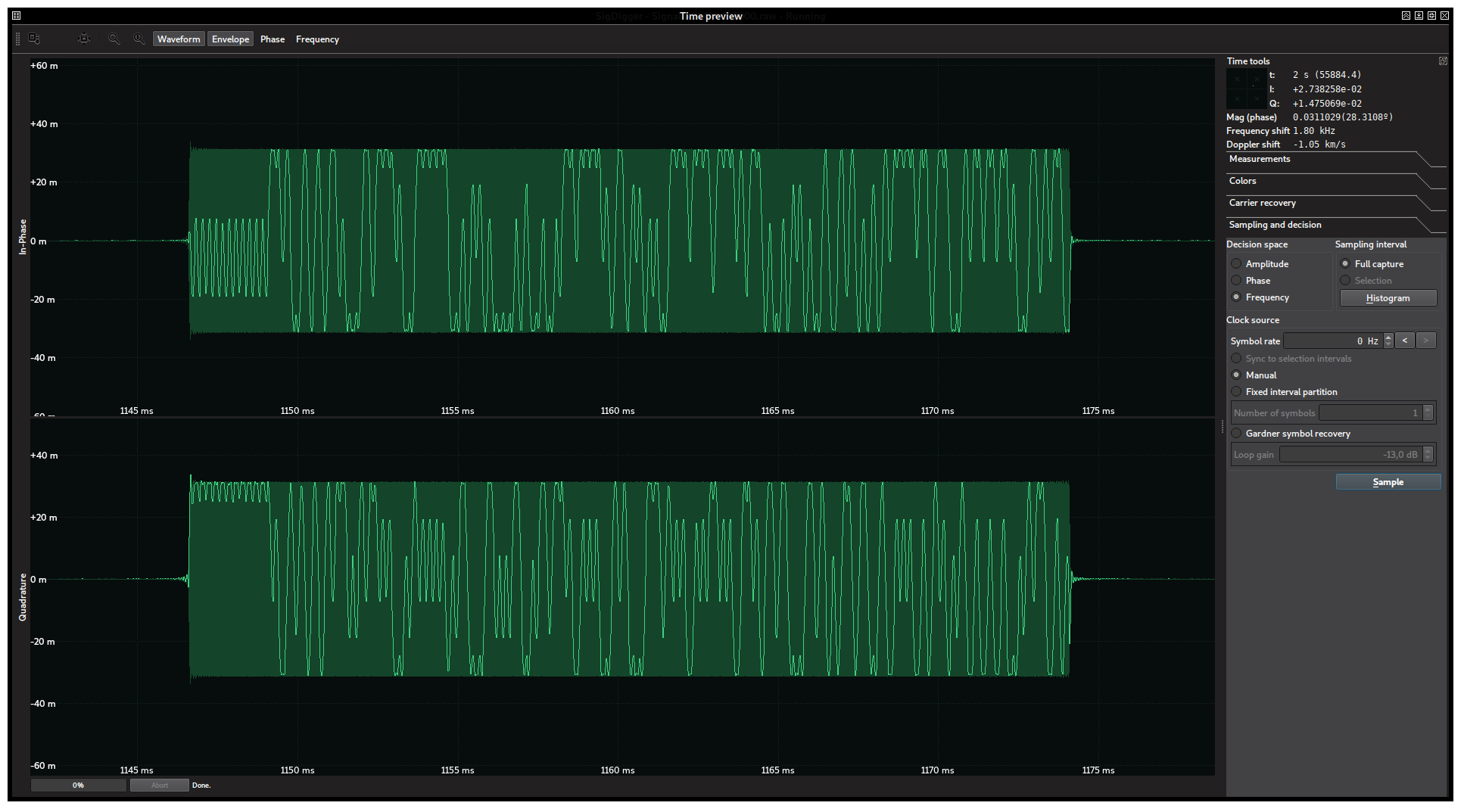
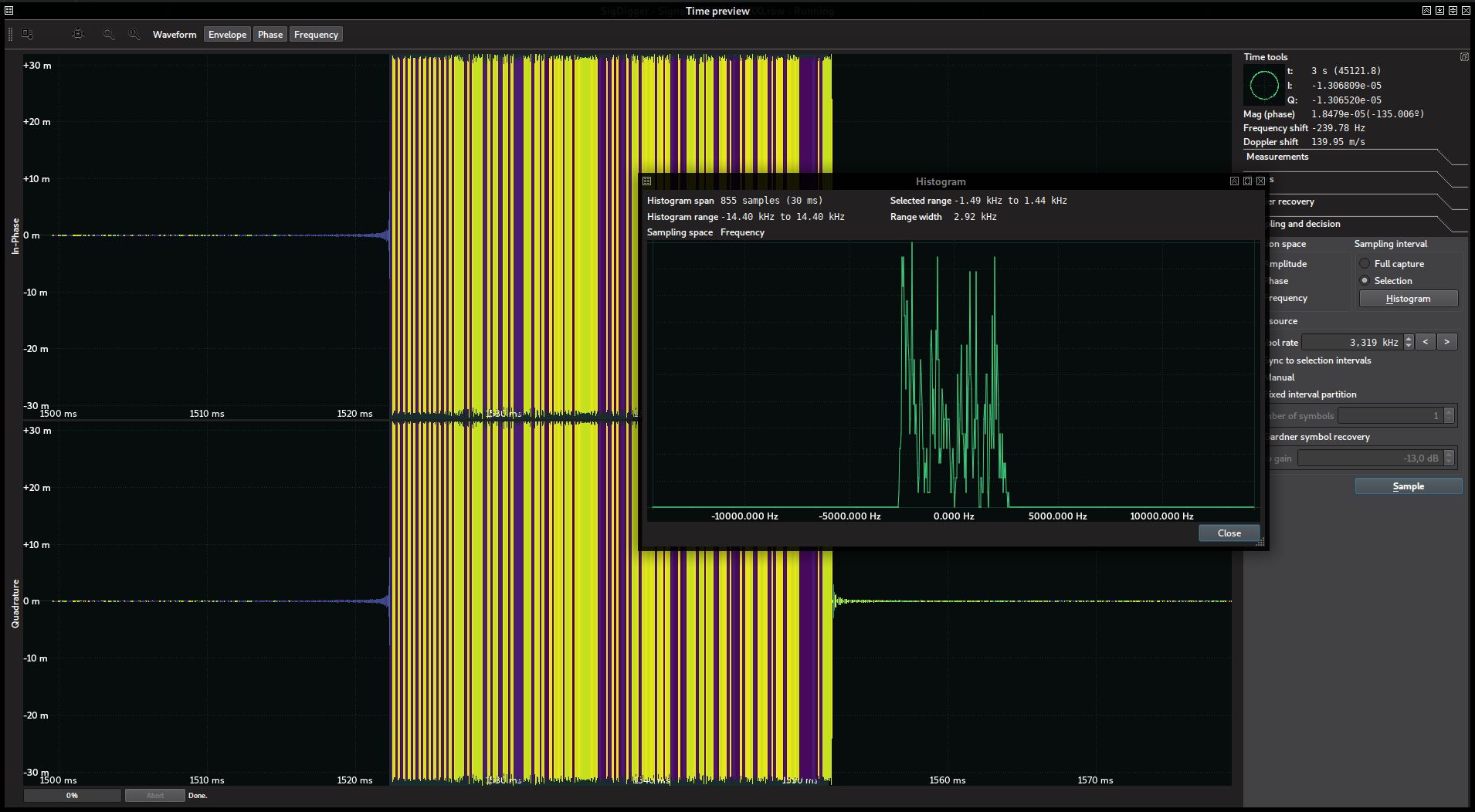
Because of its constant envelope, it must be either frequency or phase modulated. Since we are in the early stages of the contest and frequency-modulated signals are somewhat easier to demodulate than phase-modulated signals, we can go ahead and study the instantaneous frequency of the samples in the burst. To achieve this, we should go to “Sampling and decision”, choose “Frequency” as the decision space and, after making sure that the burst limits are selected in the waveform, click “Histogram”. A window like this should show up:
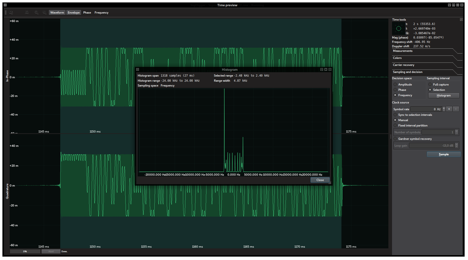
The histogram reveals that two instantaneous frequencies, roughly 4.75 Hz apart, are particularly frequent. This is strong evidence supporting frequency modulated signals. The irregular and weaker in-between peaks could be due to the pulse-shaping function and chances are that they don’t carry information at all.
In order to test our hypothesis, we can use the “Frequency” feature in the Time Window to color the wave envelope according to its instantaneous frequency.
Protip: We are about to perform precise time measurements on the signal. Although it should be sufficient to fit the filter box to the main lobe, in this particular case where other out-of-bands signals are absent and the skirt is so wide, I recommend extending the filter box to the whole spectrum (effectively increasing the sample rate of the selected channel and therefore the time resolution of the captured burst, which ultimately leads to more precise time measurements). The ide is that, although the information carried by the skirt is redundant, it contains the edges of the pulse which ultimately makes the visual inspection of the waveform clearer.
In the Time Window, we enable Envelope, Phase and Frequency, and disable Waveform. We go to “Colors”, choose a palette we are comfortable with and adjust the palette origin. Depending on the colors and the palette offset, we should see something like this:
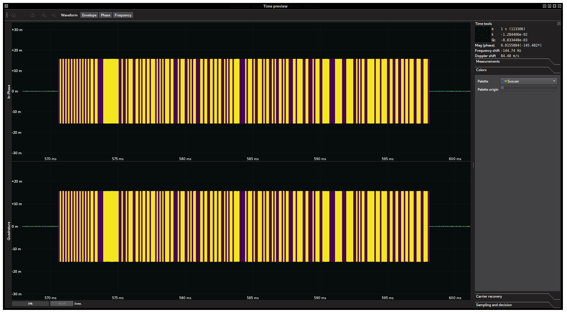
This suggest frequency-modulated pulses varying between two frequencies. The narrowest pulses are roughly the same width, suggesting a fixed symbol clock (as expected with digital signals). This hypothesis can be furtherly validated with the periodic selection feature as we did in the previous challenge. Indeed:
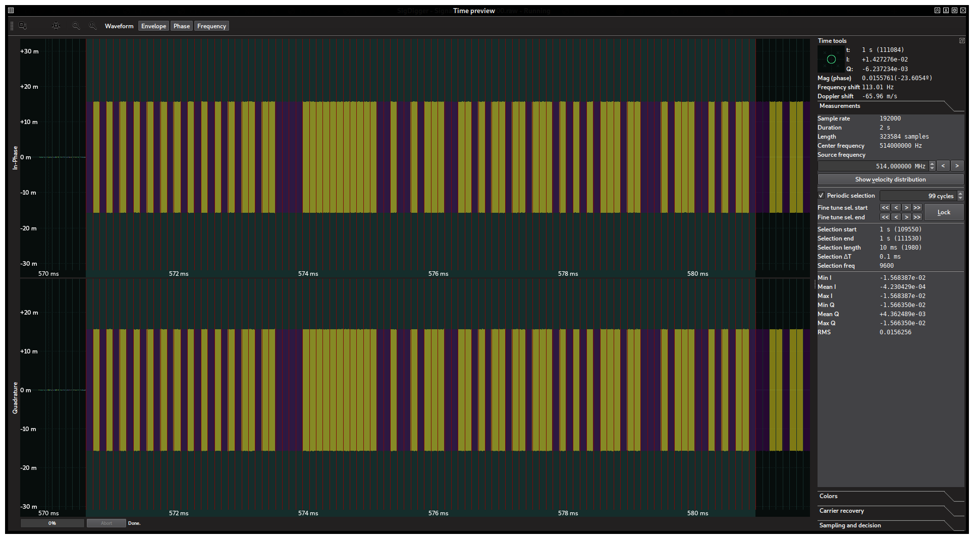
From which we can deduce it is basically 2-FSK signal at 9600 bits per second. We can go ahead and sample it as we did with our previous signal.
Note: The fact that both frequencies are 4.75 Hz apart (which is roughly half the baudrate) suggests we are dealing with MSK. Also, the long skirt suggest the presence of ISI which is a common trait of a very popular modulation named GMSK used, for instance, in GSM networks (although at a way higher rate). The gaussian filter would be the one to blame for the frequency spread of the signal.
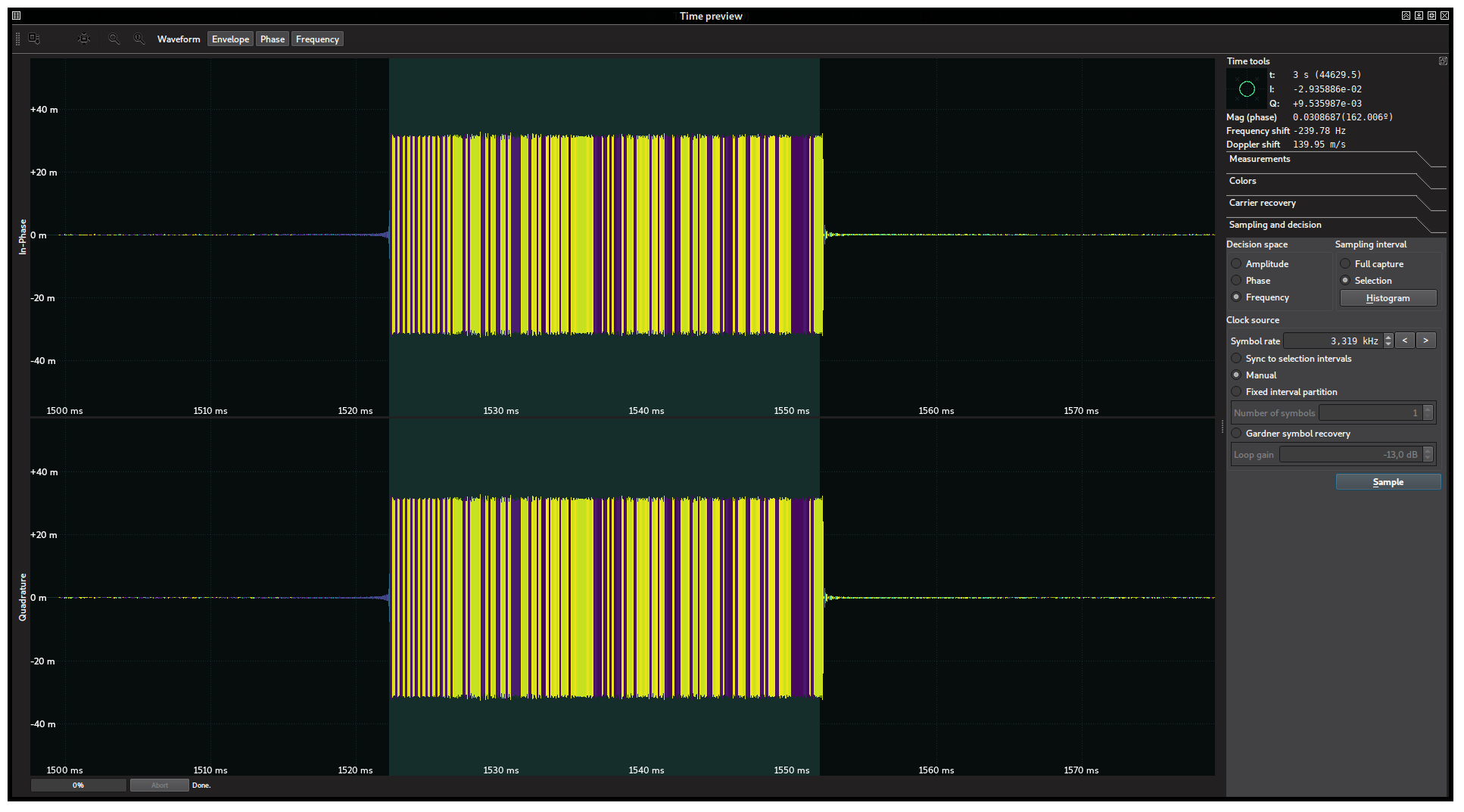
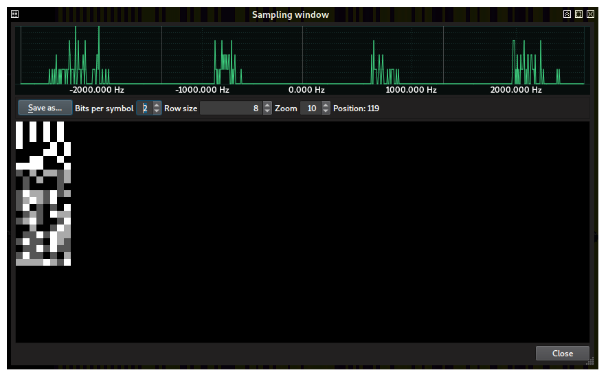
We can now select the burst with the mouse and perform a Gardner clock recovery in the frequency space. This is something we expect to work rather well due to the relatively long (24-bit) training sequence in the preamble. This time, since one frequency is negative while the other is positive, the decision threshold is exactly 0 and no further adjustments are necessary. Nevertheless, we did it for illustration purposes:
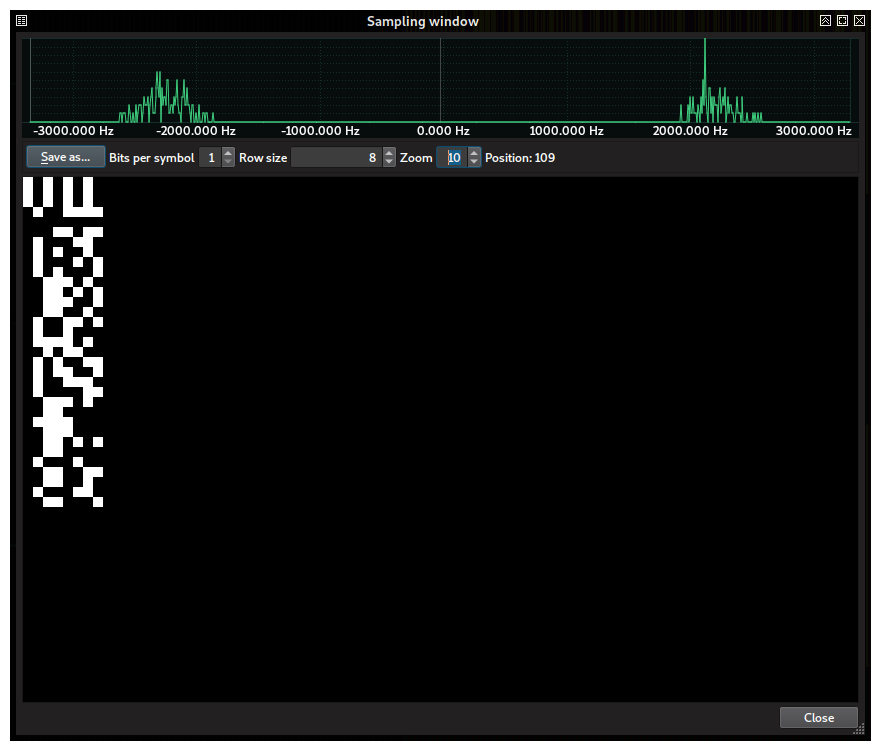
Repeating the same strategy as in the previous challenge, setting the row size to 8 shows again a row full of zeroes (in black). This is strong evidence that data is encoded in a similar fashion. By exporting the symbols to a C file and adding a function to repack the bits according to different offsets, we came up with the following code:
#include <stdint.h>
#include <stdio.h>

static uint8_t data[264] = {
  0x01, 0x00, 0x01, 0x00, 0x01, 0x00, 0x01, 0x00, 0x01, 0x00, 0x01, 0x00, 0x01, 0x00, 0x01, 0x00,
  0x01, 0x00, 0x01, 0x00, 0x01, 0x00, 0x01, 0x00, 0x00, 0x01, 0x00, 0x00, 0x01, 0x01, 0x01, 0x01,
  0x00, 0x00, 0x00, 0x00, 0x00, 0x00, 0x00, 0x00, 0x00, 0x00, 0x00, 0x01, 0x01, 0x00, 0x01, 0x01,
  0x00, 0x01, 0x00, 0x00, 0x00, 0x01, 0x01, 0x00, 0x00, 0x01, 0x00, 0x01, 0x00, 0x00, 0x01, 0x00,
  0x00, 0x01, 0x00, 0x00, 0x00, 0x01, 0x00, 0x01, 0x00, 0x01, 0x00, 0x01, 0x00, 0x00, 0x00, 0x01,
  0x00, 0x00, 0x01, 0x01, 0x01, 0x00, 0x01, 0x00, 0x00, 0x00, 0x01, 0x01, 0x00, 0x01, 0x00, 0x01,
  0x00, 0x00, 0x01, 0x01, 0x01, 0x00, 0x00, 0x01, 0x00, 0x00, 0x01, 0x01, 0x00, 0x00, 0x01, 0x00,
  0x00, 0x01, 0x00, 0x00, 0x01, 0x01, 0x00, 0x01, 0x00, 0x01, 0x00, 0x00, 0x01, 0x00, 0x00, 0x00,
  0x00, 0x01, 0x01, 0x01, 0x01, 0x00, 0x01, 0x00, 0x00, 0x00, 0x01, 0x00, 0x01, 0x01, 0x00, 0x00,
  0x00, 0x01, 0x00, 0x01, 0x00, 0x00, 0x01, 0x01, 0x00, 0x01, 0x00, 0x01, 0x01, 0x00, 0x00, 0x01,
  0x00, 0x01, 0x00, 0x00, 0x01, 0x01, 0x01, 0x00, 0x00, 0x01, 0x00, 0x00, 0x00, 0x00, 0x01, 0x01,
  0x00, 0x00, 0x01, 0x01, 0x01, 0x00, 0x01, 0x00, 0x00, 0x00, 0x01, 0x01, 0x00, 0x00, 0x00, 0x00,
  0x00, 0x01, 0x01, 0x01, 0x01, 0x00, 0x00, 0x00, 0x00, 0x00, 0x01, 0x01, 0x01, 0x00, 0x00, 0x00,
  0x00, 0x00, 0x01, 0x01, 0x00, 0x01, 0x00, 0x01, 0x00, 0x00, 0x01, 0x01, 0x00, 0x00, 0x00, 0x00,
  0x00, 0x01, 0x00, 0x00, 0x00, 0x01, 0x00, 0x00, 0x00, 0x00, 0x01, 0x01, 0x00, 0x00, 0x01, 0x01,
  0x00, 0x00, 0x01, 0x01, 0x00, 0x00, 0x01, 0x00, 0x00, 0x01, 0x00, 0x00, 0x00, 0x01, 0x01, 0x00,
  0x00, 0x00, 0x01, 0x01, 0x00, 0x00, 0x00, 0x01, };

int
main(void)
{
  int i, j;
  int p = 0;
  char b;

  for (j = 0; j < 8; ++j) {
    printf("Skip %d\n", j);
    p = j;
    b = 0;
    for (i = 0; i < sizeof(data); ++i) {
      b |= data[i] << (7 - p++);
      if (p == 8) {
        putchar(b);
        p = 0;
        b = 0;
      }
    }
  }

  return 0;
}
By compiling it and executing it in the command line, we arrive to the following result:
(metalloid) % gcc signal4.c -o signal4
(metalloid) % ./signal4 | strings
Skip 0
FREQ:592MHz,SYNC:0x850D32F1Skip 1
UUU'
Skip 2
Skip 3
Skip 4
C3$cSkip 5
UURx
1Skip 6
Skip 7
tjrd
Arriving to the flag FREQ:592MHz,SYNC:0x850D32F1, which provided us with the frequency for the next challenge.
The signal for this challenge could be found at 592 MHz, 115200 samples per second. The text accompanying the challenge was:
Once you decoded this signal, enter the flag here!
Note: This challenge will unlock a different category of challenges. So make sure to read the text of the next unlocked challenge carefully.
The signal again was in the form of short bursts every 2 seconds which, in a first glimpse, looked like a regular 2-FSK signal again:
We repeated the same procedure as in the previous challenge, arriving to a rate of 5760 symbols per second chain of demodulated bits that once grouped to bytes looked like this:
aa aa aa 85 0d 32 f1 2d 11 00 75 74 41 27 61 23 17 46 14 41 fd
Being the 3 aa the set of 24 pulses of the preamble / training sequence in the beginning of the burst and 0x850d32f1 the syncword referred in the flag of the previous challenge. These signs were assumed, in a first glimpse, to be again strong evidence that we were in the right track. However, the payload did not make any sense and struggled for hours until reaching a dead end. We had to retrace our steps to the demodulation phase and give a good look to the frequency histogram which this time looked like this:
This histogram is radically different from the one of the previous challenge. It reveals not two, but four dominant frequencies. This is strong evidence not for 2FSK but for 4FSK, this is, 2 bits per symbol.
This has profound implications in the demodulation process. To begin with, we have to select 2 bits per symbol in the Sampling Window. In this case, the correct adjustment of the decision thresholds is mandatory as every component must fall exactly in the middle of each decision interval:
If we export the data to a C file, what we get in the array is not bits but symbol identifiers (actually we were always exporting symbol identifiers, but in the previous challenges, the symbol number incidentally matched the bit it represented). Having 2 bits per symbol implies having an alphabet of 2²=4 symbols and therefore 4!=24 possible symbol-2bit translations.
In real world communications, when a symbol represents more than 1 bit, Gray coding is preferred, so the number of possible translations is actually lesser than the factorial of a power of two. In our case and due to our frustration, we wrote a code that tested all 24 possible symbol translations, packing bits with MSB first. The resulting code looked as follows:
#include <stdio.h>
#include <stdint.h>
#include <string.h>

static uint8_t data[171] = {
  0x03, 0x00, 0x03, 0x00, 0x03, 0x00, 0x03, 0x00, 0x03, 0x00, 0x03, 0x00, 0x03, 0x00, 0x03, 0x00,
  0x03, 0x00, 0x03, 0x00, 0x03, 0x00, 0x03, 0x00, 0x03, 0x00, 0x00, 0x00, 0x00, 0x03, 0x00, 0x03,
  0x00, 0x00, 0x00, 0x00, 0x03, 0x03, 0x00, 0x03, 0x00, 0x00, 0x03, 0x03, 0x00, 0x00, 0x03, 0x00,
  0x03, 0x03, 0x03, 0x03, 0x00, 0x00, 0x00, 0x03, 0x01, 0x00, 0x02, 0x00, 0x02, 0x02, 0x01, 0x02,
  0x00, 0x01, 0x00, 0x02, 0x00, 0x00, 0x01, 0x02, 0x00, 0x01, 0x00, 0x00, 0x00, 0x00, 0x01, 0x00,
  0x01, 0x03, 0x02, 0x02, 0x01, 0x03, 0x01, 0x02, 0x01, 0x02, 0x03, 0x02, 0x01, 0x03, 0x00, 0x00,
  0x01, 0x03, 0x00, 0x01, 0x00, 0x01, 0x00, 0x03, 0x00, 0x01, 0x02, 0x01, 0x00, 0x03, 0x02, 0x02,
  0x01, 0x02, 0x03, 0x01, 0x00, 0x00, 0x01, 0x03, 0x00, 0x00, 0x02, 0x00, 0x00, 0x01, 0x03, 0x02,
  0x00, 0x01, 0x01, 0x03, 0x01, 0x03, 0x02, 0x02, 0x01, 0x03, 0x01, 0x01, 0x00, 0x03, 0x02, 0x01,
  0x00, 0x01, 0x01, 0x03, 0x01, 0x03, 0x01, 0x01, 0x01, 0x03, 0x01, 0x01, 0x00, 0x01, 0x00, 0x02,
  0x02, 0x02, 0x02, 0x02, 0x03, 0x02, 0x01, 0x03, 0x00, 0x00, 0x00, };

uint8_t buffer[173];

int dicts[24][4];

void
swap(int *a, int *b)
{
  int tmp;

  tmp = *a;
  *a  = *b;
  *b  = tmp;
}

void
compose_dicts(void)
{
  int map[4] = {0, 1, 2, 3};
  int i, j, k, l;
  int n = 0;

  for (i = 0; i < 4; ++i) {
    swap(map + i, map + 3);

    for (j = 0; j < 3; ++j) {
      swap(map + j, map + 2);

      for (k = 0; k < 2; ++k) {
        swap(map + k, map + 1);

        memcpy(&dicts[n++][0], map, 4 * sizeof(int));

        swap(map + k, map + 1);
      }

      swap(map + j, map + 2);
    }
    swap(map + i, map + 3);
  }
}

size_t
compose_buf(int dict, int offset)
{
  int q = 0;
  uint8_t b = 0;
  int i;
  size_t len = 0;

  for (i = offset; i < sizeof(data); ++i) {
    b |= dicts[dict][data[i]] << (6 - q);
    q += 2;

    if (q == 8) {
      buffer[len++] = b;
      b = q = 0;
    }
  }

  return len;
}

int
main(void)
{
  int i, off;
  size_t len;

  compose_dicts();

  for (off = 0; off < 4; ++off) {
    for (i = 0; i < 24; ++i) {
      len = compose_buf(i, off);
      fwrite(buffer, len, 1, stdout);
    }
  }

  return 0;
}
By compiling and running again, this time grepping by FREQ to get rid of all the non-relevant garbage:
(metalloid) % gcc signal5.c -o signal5
(metalloid) % ./signal5 | strings | grep FREQ
FREQ:2.54GHz,SYNC:0xC00F
Which led us to the flag FREQ:2.54GHz,SYNC:0xC00F.
The frequency of the previous challenge ended up being useless, as the text for the unlocked challenge was the following:
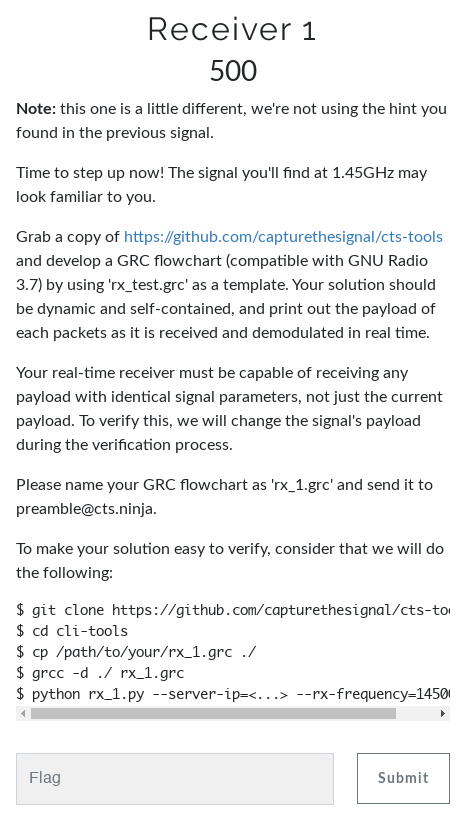
The signal in 1.45 GHz was exactly like the one in the third challenge, OOK at 10 bits per second, with a 2-bit length field after the syncword. However, it was Friday night already, GnuRadio (both 3.7 and 3.8) refused to work in my computer and had to use GR 3.7 that was installed by chance on a different computer. In any case, after lots of trial-and-error, we arrived to a flowgraph that aligned the bit stream to the syncword and dumped everything to the standard output that ended up not being accepted because it didn’t take the length into account.
It was fun to participate in a CTF focused only on radio signals. I’ve been doing this a lot lately with real world signals, but I also wanted to test SigDigger in an environment in which signals are made to be difficult to understand. Regarding SigDigger, it is clear that there’s a lot of UX improvements that have to be done if I want it to be a real world alternative to existing software.
Regarding the CTF itself, it was a bit frustrating to be forced to use a legacy version of a software whose instability and lack of documentation made me code my own DSP library and blind signal analysis software from scratch back in 2016. In this particular scenario, writing an OOK signal demodulator could have been done in an extremely short C program, featuring an AGC and a simple threshold-based decider measuring pulse widths. Increased noise immunity could be achieved with a more elaborate matched filter and clock recovery algorithm like M&M or Gardner’s although according to the text of the Receiver 1 challenge seemed to be kind of an overkill.
I’d love to see more contests like this in the future, and I think it was a hell of a breakthrough bothering to make it remote. A lot of ideas came to my mind while solving the challenges. Hope they inspire someone (and, who knows, I may even work in some of them):
Anyways, I think the overall experience was fun and I’m looking forward for future editions of this CTS.
Stay tuned!