
BatchDrake
Hacking, HAM Radio (EA1IYR), DSP, physics and more
Hacking, HAM Radio (EA1IYR), DSP, physics and more
Hi, everyone! It’s been a while since my last blog post here. I couldn’t help it: I began a master’s degree in Astrophysics in the UCM last year, and a lot has been going on since then. In particular, I had an assignment for the subject Extragalactic Astrophysics, consisting on a scientific poster based on a freely chosen paper out of a list provided by the teacher.
One of the papers in the list was Measurement of the flux density of Cas A at 4080 Mc/s by Arno Penzias and Robert Wilson. This paper is particularly interesting for two reasons: first, this is the paper that led to the discovery of the Cosmic Microwave Background. Spoiler alert: they measured Cassiopeia A flux at 4 GHz successfully, being ~1 kJy, overestimaing its secular dimming to 1.1% per year. Second, it talks about radioastronomy in 4 GHz, and as we all know, radio is inherently fun.
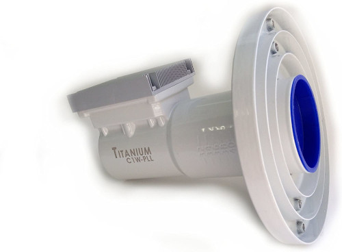
From the hobbyist perspective, 4 GHz radioastronomy is especially relevant for economic reasons: bright unresolved sources (~0.5 kJy, namely Cas A and Cyg A) are visible from the northern hemisphere and, since 4 GHz is in the middle of the portion of the C Band allocated to satellite TV, cheap reception equipment must exist. In particular, COTS C-Band LNBs can be bought almost anywhere. A quick search in Amazon “LNBF C Band” shows C-Band LNBs with prices as cheap as 16 € and excellent figures:
Of course, an LNB alone is of little use. We need an appropriate parabolic reflector in order to get an usable beamwidth. According to this online calculator, dishes as small as 120 cm with a 0.65 efficiency have a 3 dB beamwidth of 4.22º.
The question arises almost naturally out of these numbers: can I reproduce Penzias & Wilson experiments at home?
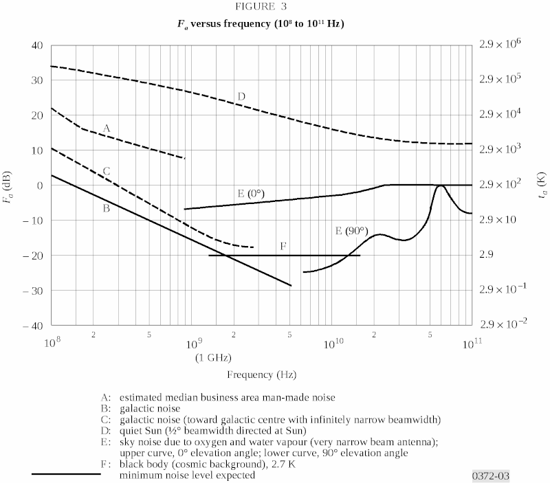
Let’s start by calculating a rough estimate of the order of magnitude of the power increment due to the presence of Cyg A/Cas A with respecto to the background sky noise. According to this graph, we could assume that the background noise is dominated by the CMB at 2.9 K and 4 GHz. But since both Cyg A and Cas A are rather close to the galactic plane, we’ll be a bit more pessimistic and extend the C curve horizontally, rising the floor up to 15 K:
The power spectral density (PSD) at the LNB output when the beam (including all its sidelobes) covers a fixed-noise temperature region in the sky can be naively modelled as Johnson-Nyquist noise by:
\[S_b=\frac{dP}{d\nu}=G(k_BT_{n}+k_BT_{s})\]With $k_B$ the Boltzmann’s constant, $T_n$ the typical noise temperature of the LNB’s low noise amplifier, $T_s$ the noise temperature of the sky and $G$ the gain of the LNB. Easy, right?
The truth is that this formula rarely holds. Antennas are not perfect, and their sidelobes pick a lot of surrounding noise. This phenomenon is called spillover, and implies that only a (hopefully big) fraction of the power entering the internal low noise amplifier will actually come from the sky. If we assume that the surrounding noise is purely thermal in nature and caused by the ambient temperature of the objects close to us (buildings, trees or the floor itself), we can introduce the parameter $\alpha$ describing the amount of spillover of our antenna. If $T_{amb}$ is the ambient temperature, a more realistic model could be:
\[S=\frac{dP}{d\nu}=Gk_B\left[T_{n}+(1-\alpha)T_{s}+\alpha T_{amb}\right]\]$S$ will be our background sky level (in terms of PSD) as seen at the output of the LNB. In general, the power spectral density for astronomical sources is rather white (i.e. flat), even if we consider the typical bandwidths (~3 MHz) supported by low cost SDR receivers.
Now let’s consider what happens to the output PSD if our antenna is perfectly oriented towards a point source like Cas A or Cygnus A (with angular sizes way below 1º). Since these sources are rather small and/or irregular, and therefore difficult to characterize in terms of temperature and angular diameter, we will take instead their spectral irradiance (also known as flux density) into account. This quantity describes the noise PSD coming from a distant source per unit of surface which, in the field of radioastronomy, is usually measured in Janskys ($1\text{ Jy}=10^{-26}\text{W}\text{m}^{-2}\text{Hz}^{-1}$). The PSD collected by the antenna is related to the spectral flux $F$ by the antenna aperture $A$:
\[\frac{dP}{d\nu}=AF\]For both Cas A and Cyg A, the order of magnitude of the spectral flux is 500 Jy. In parabolic antennas, the antenna aperture is related to the dish area by a dimensionless factor called aperture efficiency, which describes how much of the received power is actually collected by the dish with respect to its physical size. We’ll call this factor $\eta$:
\[A=\eta A_d=\frac{1}{4}{\eta \pi D_d^2}\]With $D_d$ the diameter of the dish. A typical value for the aperture efficiency of dish antennas is 65%, but we’ll be somewhat conservative here and give it a more modest 50%. Then, the power spectral density increment due to this source can be approximated by:
\[\Delta S=\frac{1}{4}G\eta \pi D_d^2F\]In the field of SDR and radio receivers in general, it is customary to measure power levels in dB. Since dBs describe a logarithmic scale, the observer will detect a power increase at the output of the LNB of:
\[\Delta S_{dB}=10\text{log}_{10}\left(S+\Delta S\right)-10\text{log}_{10}(S)=10\text{log}_{10}\left(\frac{S+\Delta S}{S}\right)\]Which is a quantity that does not depend on the gain, but on all noise components. Now, let’s see how $\Delta S_{dB}$ behaves on a typical (mostly suboptimal) setup:
Injecting these values in the above expression yields a poor 0.004 dB increment in the noise output. By reducing the spillover loss to 0.1, the increment nears 0.01 dB. Still low, but as long as the standard deviation keeps equally low, we would be able to detect them. Ideally, we could integrate the output a lot (either by increasing the bandwidth or the integration time, or even both) in order to reduce the fluctuations and get a more or less significant detection. The question is, will a LNB designed to receive satellite TV cooperate with us?
In the next chapter, I’ll describe my experiments with a typical C-Band LNB and explain why things are not as easy as they seem.
Stay tuned!