
BatchDrake
Hacking, HAM Radio (EA1IYR), DSP, physics and more
Hacking, HAM Radio (EA1IYR), DSP, physics and more
Alright, so earlier last summer I managed to gather all the necessary parts for my DIY C-Band radiotelescope. My initial goal was to buy a primary focus dish somewhere near Madrid. Unfortunately, those are extremely difficult to find in Spain because reasons, at least at a reasonable price. I had to switch to plan B, this is, a medium-sized 110x120 cm offset antenna that was eventually purchased from diesl for an extremely reasonable amount (65€). Since the LNB is designed for primary focus dishes, I had to buy a conical scalar ring so that the dish was completely illuminated (hence reducing spillover losses to a minimum).
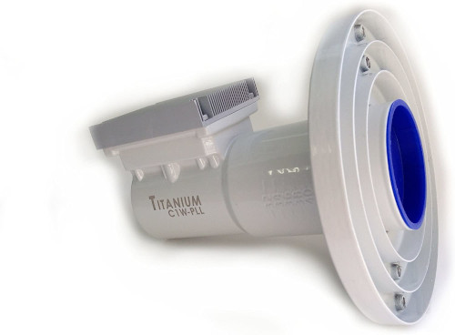
The LNB I ended up purchasing was the Titanium C1-PLL because of its integrated WiMax/LTE/WiFi notch filters. Man-made radio interference is one of the biggest threats to radioastronomy in general, and it is rather easy to saturate a 65 dB amplifier with the (seemengly) faintest undesired signal.
Another reason why I ended up buying this one was it is PLL-driven. Compared to the cheaper DRO-based LNBFs, frequency stability of PLL-based LNBs is in general terms better than that of its DRO-based alternatives and somewhat more resistant to aging. For this application, frequency stability is not critical (we are measuring the PSD of a rather flat signal, and therefore frequency drifts will be barely noticeable). However, since radioastronomy is only one of my side projects and, in general (but especially for radio), cheap is expensive, I decided to spend more money in something durable.
And regarding the receiver part, I relied on my beloved AirSpy Mini as usual.
It is important to recall how sat TV LNBs work before going on. LNBs are basically amplified downconverters plugged to a pair of perpendicular switchable antennas and optional filters. For C-band LNBs, the downconverter is implemented as a mixer plugged to a local oscillator running at 5150 MHz. This means that the mixing products of a 4 GHz signal will be at 9150 MHz (which is filtered) and -1150 MHz. The minus sign means that the spectrum of the mixing product will be reversed with respect to the original signal. Compare it to the typical Ku-band LNB, which mixes a 9750 MHz LO with a 10.7 GHz input signal, getting the lower mixing product in 950 MHz (positive). Reversing the spectrum affects the phases of the signal but not its amplitudes, and therefore has no effect on its PSD either.
TV LNBs are supplied directly from the coaxial cable with a DC current injected by the receiver box. The LNB uses the value of the supply voltage to switch between two perpendicularly polarized monopoles: supply voltages of $12\pm2\text{ V}$ select the vertically-polarized monopole while supply voltages of $20\pm4\text{ V}$ select the horizontally-polarized one. In both cases, the supply voltage is way too high compared to what my little AirSpy Mini can rise, and therefore a standalone bias T will be necessary. Finally, since 12 V is enough to power the LNB in vertical polarization mode, a regular car battery will just do the job.
I received my first light in late June 2020, after a precarious setup out in a park near my apartment.
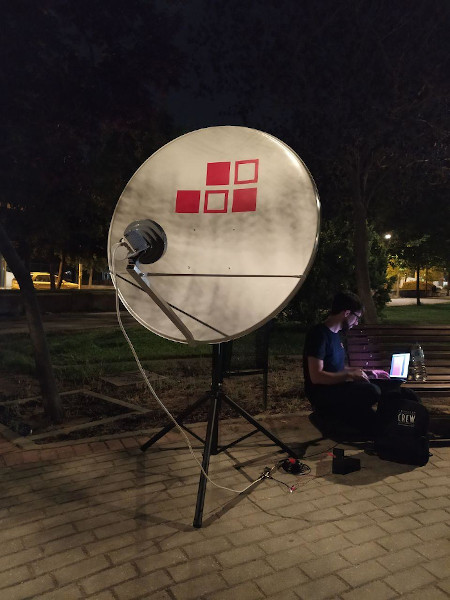
Neededless to say, the results were a bit disappointing because of the buildings blocking most of the sky, but at least I could conclude something: trees and buildings are indeed warmer than the sky in 4 GHz.
After that first light, I was ready to perform power measurements. I coded a new graphical tool named RMSViewer inside SigDigger that, along with suscli’s rms subcommand, allowed me to plot power measurements in arbitrary units coming from a previously configured signal source. First results from my window were promising as I could detect cars passing in the street: their low emissivity in 4 GHz reflected the blackness of the sky, showing up as brief valleys in RMSViewer’s power plots.
The next step was to perform a study of the effect of the temperature on the LNB after a 12 hour observation to a fixed point. In order to do this, I rigged up a USB controlled temperature sensor by plugging an I2C GY-906 IR temperature sensor (thanks, DigitSpace!) to an Arduino Nano, with the IR sensor pointing directly to the heatsink. Of course, due to the low emissivity of the aluminium the heatsink was made of, I had to isolate the sensor from the surroundings with a small tin box.
Embedded inside the GY-906 and in addition to the IR sensor, an ambient temperature sensor is also provided. A small C program read both temperature recordings and dumped them to a plain text file.
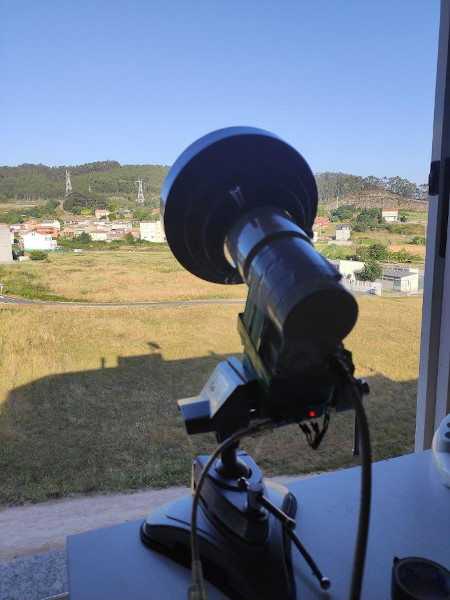
The experiment was carried out in Andrés Pérez’ apartment by pointing the LNB to the sky. I didn’t care too much about the angular resolution, I was only hoping that some of the thermal noise of the landscape got into the beam, and use it to make an estimate of the beamwidth of the LNB alone.
The results could have not been more baffling:
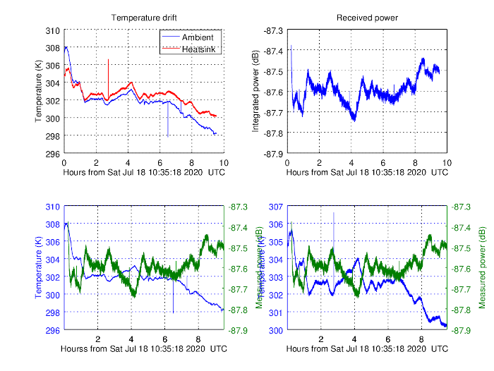
I was expecting the PSD to increase with temperature, while I was observing exactly the opposite effect! What could be going on in here?
When the novice wants an amplifier to increase the power of a radio signal, usually thinks of some magic device that performs the following operation on the signal:
\[y(t)=Gx(t)\implies \frac{dP_y}{d\nu}=G^2\frac{dP_x}{d\nu}\implies P_y=G^2P_x\]With $G$ the gain of the hypothetical amplifier (in linear scale), which would increase the output power $G^2$ times.
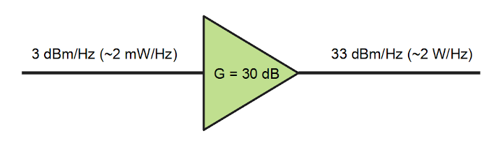
This does not exist. Amplifiers are not perfectly linear (so say goodbye to the product operation), inject noise, are band-limited, their frequency response is not necessarily flat and their gain depend on the temperature. Even if the signals are sufficiently weak so that the amplifier is kept in the linear region, a more accurate model of the output power could be the following:
\[\frac{dP_y}{d\nu}=G^2(T,\nu)\left[\frac{dP}{d\nu}+k_BT_n\right]\]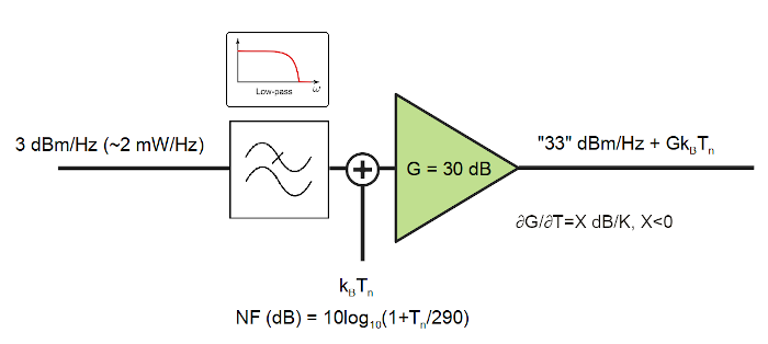
I basically discovered that $\frac{\partial G}{\partial T}<0$ the hard way. Using linear regression, I could estimate a gain to temperature slope of $-0.1\text{ dB/K}$, which I attempted to use to compensate for these gain fluctuations. The results after the correction were still disappointing:
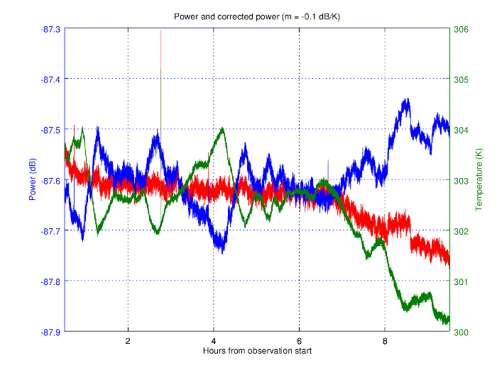
Although most of the fluctuation was compensated, there were power variations that I could not be sure whether they came from the sky or an unstable gain. In any case, the fluctuations were big, even after increasing the integration time (0.05 dB was still too big). I had to find another way.
It seemed almost impossible to control those hidden variables that were affecting the amplifier back then, until something I read in Penzias & Wilson’s paper came to my mind: Holmdel’s radiotelescope used a half-wave plate and two rotary joints to switch between a reference noise signal (like a helium-cooled cold load inside a dewar) and their horn antenna. This trick is called Dicke switch and is used in many radiotelescopes to compare noise levels.
As mentioned earlier, LNBs are able to switch between two antennas. How about leveraging the existing circuitry to create a DIY Dicke Switch?
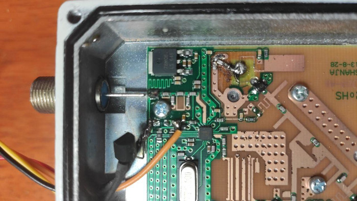
The idea would be the following: if an RF switch is right before the amplifier, I could get rid one of the monopoles and replace it by a matched resistor that would inject thermal noise, whose power spectral density can be well approximated by a Johnson-Nyquist noise ($k_BT$). Assuming a mostly-constant temperature, I could use the noise reference power to normalize the signal power and get rid of undesired gain effects. Let’s give a look to the LNB’s PCB:
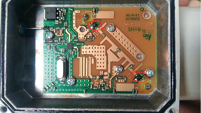
Circled in red are two GaAsFET HEMTs used both for switching and amplification. They are both the LNA and the RF switch: when one is polarized, it acts as an amplifier while the other remains in cut-off state. Switching happens by lowering the voltage of the corresponding gate terminal with respect to ground. This leads to a few drawbacks:
On the other hand, polarization detection is performed trivially by means of a zener diode (reddish crystal cylinder next to the screw on the up-left corner). Voltage measurements of this zener diode under both supply voltages revealed that it was connected to a voltage divider, producing an almost 0 V level for vertical polarization and 3 V for horizontal polarization. These are TTL levels I could control with another Arduino Nano!
With all this information in hand, the roadmap for the LNB modification was:
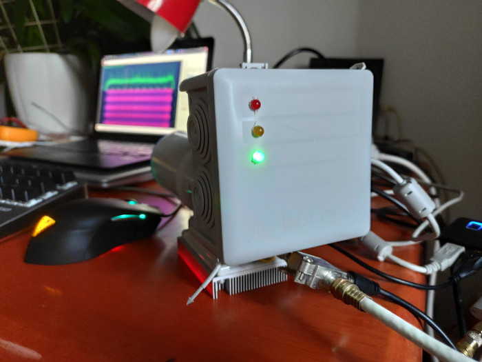
And after a couple of afternoons, the modified LNB looked like this:
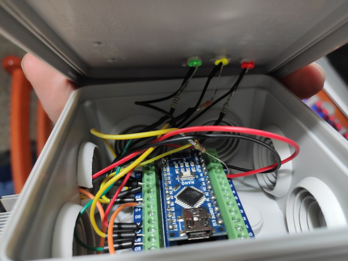
The Dicke switch logic and control was implemented in a small Arduino Nano program I carefully put in a watertight box with three LEDs indicating what the circuit was doing (antenna selected, reference selected and measuring temperature).
And this is what the finished LNB looks like. Note SigDigger’s alternating spectrogram. Computers are extremely bright in 4 GHz (surprise!).
More testing was carried out by filling the LNB entry with RF absorber and observing both ambient temperature and LNB physical temperature in 24 hour cycles:
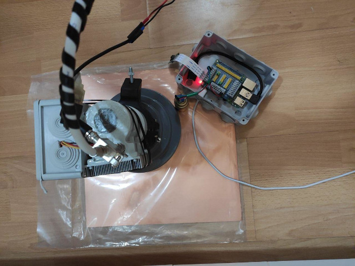
A small C program was coded to control the Dicke switch, take measurements, normalize them and output the results to a MATLAB’s /mat file. The comparison between the antenna and reference was promising:
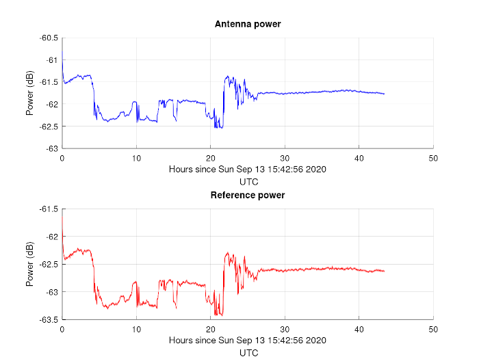
And the normalized power was even more promising:
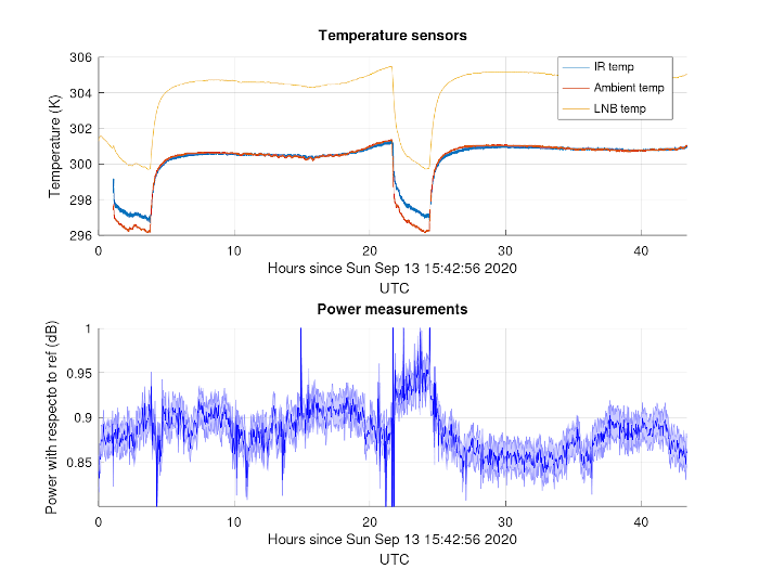
Long-term fluctuations of 1 dB were reduced to 0.1 dB. And even 0.02 dB for short term observations. Long term fluctuations were difficult to explain, but I’d point the finger at different thermal inertias of both GaAsFET. We are not in the 0.01 dB minimum yet, but we are close.
In the next post, I’ll share my first real-world observations and future work on this project.
Stay tuned!
This experiment was made possible thanks to the sponsorship of DigitSpace. Check it out!