Measuring mesospheric winds with GRAVES

Last weekend I managed to plug the J-Pole antenna I built this summer to my recently acquired Yaesu FT-817 and tune it to hear GRAVES radar reflections at 143.050 MHz. But, what is GRAVES, to begin with?

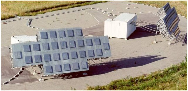
GRAVES is a French space surveillance system, consisting of a bistatic radar in which the transmitting station uses 4 phased arrays covering 180º of the south of France. Each phased array scans a 45º-width sector simultaneously along with the others, with a horizontal beamwidth of 7.5º and discrete angle steps (6 in total). A full scan cycle takes 19.2 seconds before restarting again.

Although initially designed to detect NEO spacefracts and determine their orbital elements, its power allows amateurs to monitor its reflections and test meteor scatter effectivity during meteor showers (with some particularly impressive results during prolific meteor showers like Perseids every summer).

As an amateur, I decided to play a little with it and ended up doing some interesting homemade science on the gathered data. Let’s start!

The physics of meteor trails

What is popularly known as meteor is actually what an object in outer space named meteoroid turns into when it enters Earth’s atmosphere. Meteoroids are pretty much like asteroids, but smaller (up to one meter wide) and way more numerous. During the fall of a medium-sized meteoroid (i.e. bigger than 10cm) through the atmosphere of our planet, its kinetic energy is gradually transformed into heat as it compresses the air in front of it. It is this region of compressed and heated up gas what gets ionized and glows. When this happens, the meteoroid becomes a meteor.

These events take place where the atmospheric density is high enough: typically in the mesosphere, around 75-100 km above the ground. As the meteor passes, a strched cloud of temporarily ionized gas is left behind (named ionization trail). Since the ionization trail is basically a plasma, it also has a defined plasma frequency. Roughly speaking, the plasma frequency tells us what is the maximum radio wave frequency a plasma can reflect. For cold plasmas like these, the plasma frequency is function of its (free) electron density:

\[f_p=\sqrt{\frac{n_ee^2}{4\pi^2m_e\varepsilon_0}}\]

Where \(n_e\) is the electron density, \(e\) the electric charge of a single electron, \(m_e\) the effective mass of the electron and \(\varepsilon_0\) the vacuum permitivity. In SI units, this expression can be approximated to:

\[f_p=8.98\sqrt{n_e}\]

According to the article Characteristics of Radio Echoes from Meteor Trails: I. The Intensity of the Radio Reflections and Electron Density in the Trails by A. C. B. Lovell and J. A. Clegg:

The results show that the density in the trail of a 5th magnitude meteor (on the limit of naked eye visibility) is approximately \(2\times10^{10}\) electrons per cm. path Brighter meteors (similar magnitude + 1) produce \(10^{12}\) electrons per cm. path.

Which leaves the question of the dimensions of the trail section unanswered (however, this value alone is still useful for \(\lambda\) much greater than the dimensions of the meteor, as it allows to perform calculations about the magnitude of the scatter). For VHF frequencies, where \(\lambda\) is of the order of 1m, this is not enough anymore, and we need information about the true electron density.

According to this article, meteor trails are usually categorized as “overdense” and “underdense”, whith typical electron densities for overdense meteors of the order of \(10^{14} m^{-3}\). This gives a plasma frequency of:

\[f_p=8.98\sqrt{10^{14}\text{ m}^{-3}}=89,8\text{ MHz}\]

Which corresponds to the lower part of the VHF band. Since GRAVES works at 143.050 MHz, reflection will happen at densities above:

\[n_e>\left(\frac{143,050\cdot10^6}{8,98}\right)^2=2,54\cdot10^{14}\text{ m}^{-3}\]

This means that GRAVES will reflect only those trails that are clearly overdense.

Dust in the (mesospheric) wind

The mesosphere is far from being a stagnant part of the atmosphere. Depending on the latitude and the season, its wind speed profile may peak around tens of m/s and some Doppler shift may be observed during these echoes.

One can think of taking this Doppler shift directly to calculate the speed at which the ionization trail is moving. However, this is not as straightforward as it seems, because I can only use GRAVES as a bistatic radar, with the transmitter station located in Broye-les-Pesmes and the receiver station in my apartment in Madrid.

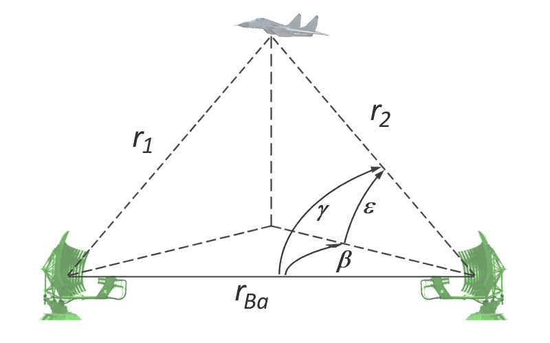
Structure of a typical bistatic radar. The transmitting and receiving antennas are separated by a fixed distance \(r{Ba}\). Image by Wikipedia user Charlie Wisky, downloaded from https://commons.wikimedia.org/wiki/File:Bistatic_Radar.png_

Doppler shift in bistatic radars is more difficult to deal with. Since the radar signal hits the trail in one direction and bounces it back to the receiver in another direction (actually, it is scattered in all directions), two Doppler shifts will overlap and may partially cancel each other:

\[\Delta f=\lambda^{-1}\left(v_T+v_R\right)\]

In particular, if the relative speeds of the ionization trail \(v_T\) and \(v_R\) are the same in magnitude but opposite in sense from both perspectives (transmitter and receiver), the measured Doppler shift will be zero. Highest degrees of cancellation will happen with meteors occurring between both stations and near their mutual line of sight. On the other hand, meteors occurring outside the space between both stations will in fact add their shifts up. In general, we expect Doppler shifts in the range:

\[\Delta f \in [0, 2\lambda^{-1}v_{\text{max}})\]

With \(v_{\text{max}}\) being the maximum relative mesospheric wind speed, measured from the ground. The boundary \(2\lambda^{-1}v_{\text{max}}\) refers to the extreme case where the reflection occurs infinitely far away (or in the line of sight between both stations but outside the region in between, which is impossible in this case due to the vertical angle of GRAVES antennas), and therefore we would expect frequencies way below this value.

Conversely, if the Doppler shift is given, we can deduce that:

\[v_m\geq\frac{\lambda}{2}\Delta f\]

With \(v_m\) the mesospheric wind speed in the ionization trail.

Retrieving and analyzing data

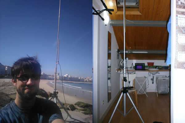
How does all of this connect with reality and how do we actually measure Doppler shifts? First, we will need some nice VHF SSB receiver (my Yaesu FT-817ND did the job, but some people out there made it with a RTL-SDR) and a vertically polarized VHF antenna, preferably centered around 143 MHz. Mine was a homemade J-Pole antenna I built this summer with copper tubes bought in Brico-Depôt, whose construction details I refrain from explaining. It was pretty cumbersome, but seemed to be enough for this experiment:

Since most frequency shifts will fall in the audible range, I can simply plug the audio output of my Yaesu to the soundcard’s input and record everything with Audacity. After tuning my receiver to 143.049 MHz USB (to make the echoes audible at 1000 Hz and leave some room for shifts), I realized that most echoes will not shift more than 30 Hz from their central frequency and will last for at least 77 ms.

With these results in mind, we can now retrieve the Doppler shift by doing dome DSP. It turns out that a frequency shift of a pure sine wave (as GRAVES signal) is equivalent to frequency-modulated signal, and therefore we can apply a quadrature demodulator on it to calculate the magnitude of the shift.

Let’s start by re-centering the spectrum in 1000 Hz and applying a low-pass filter with cutoff frequency 30 Hz on it:

\[y[n] = h_\text{LPF}[n]*\left(e^{-j2\pi\frac{1000}{f_s}n}x[n]\right)\]

The low-pass filter is used to isolate the positive from the rest of components of the signal (especially from its image and some spurs around DC that I think are my soundcard’s fault). Now, we can do quadrature demodulation normally:

\[\Delta f[n] = \frac{f_s}{2\pi}\text{arg}\left(y[n]\bar{y}[n-1]\right)\]

Which will return zero if and only if the Doppler shift is zero. For discrete signals, the argument of the product \(y[n]\bar{y}[n-1]\) equals to the instantaneous angular frequency of the signal. The scaling factor \(\frac{f_s}{2\pi}\) converts the normalized angular frequency to the absolute frequency of the shift in Hz. Of course, the validity of this result depends on the instantaneous SNR too.

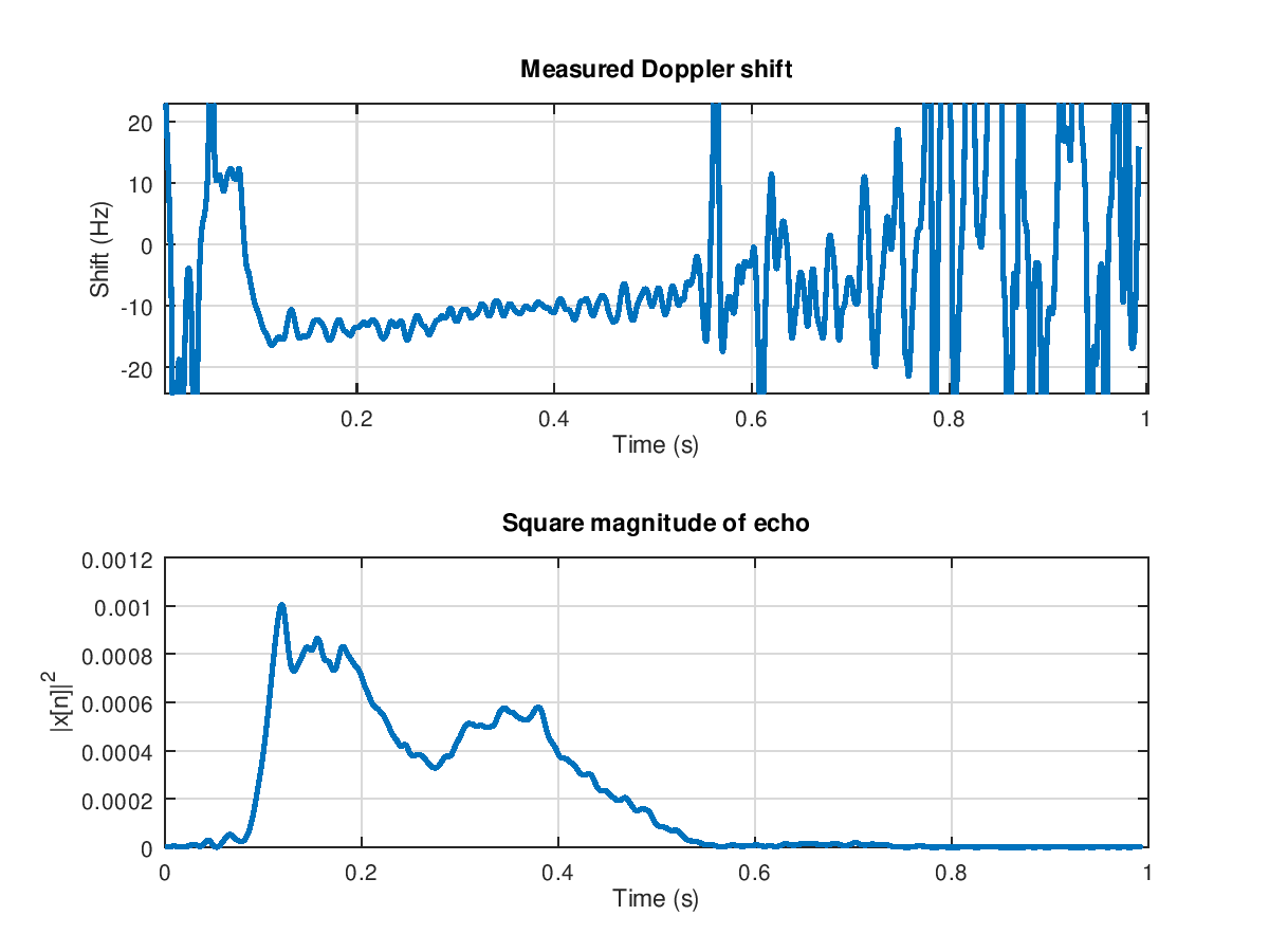
Measured Doppler shift of a particularly strong GRAVES echo. As the echo fades away, our measure of the Doppler shfit becomes progressively unreliable. However, an almost linear variation of the shift’s value can still be noticed. This may imply fast local variations of mesospheric wind speed.

Turning this Doppler shift into wind speed directly is not directly possible, as it depends on the reflection angle, wind direction, etc. However, it still can be used to compute a lower bound of the actual wind speed. Doppler calculations on the loudest echoes suggested wind speeds above 30 m/s. This is consistent with previous experimental results, in which mesospheric wind speeds are of the order of tens of m/s:

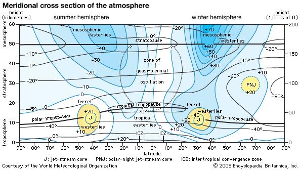
Meridional cross section of the atmosphere to a height of 60 km (37 miles) in Earth’s summer and winter hemispheres, showing seasonal changes. Numerical values for wind are in units of metres per second and are typical of the Northern Hemisphere, but the structure is much the same in the Southern Hemisphere. Positive and negative signs indicate winds of opposite direction. © Encyclopædia Britannica, Inc.

Making it automatic

Selecting and isolating samples by hand using Audacity is boring, and although short and weak echoes are common, it may take hours for a loud echo to show up. In the mean time, the capture file gets bigger and bigger, slowly consuming the free space of our hard drive.

Since I don’t consider myself a patient person, I came up with an algorithm that dynamically computes the SNR of the received signal and, by means of a moving average, looks for sudden increases in power level. The output is a boolean signal, indicating whether we are in the middle of an echo or not. The algorithm looks like this:

All signal buffers are initialized to 0.
Let \(\tau\): length (in samples) of the shortest echo (77 ms)
Let \(f_G\): frequency offset at which the radar is tuned (1000 Hz)
Let \(f_1\): cutoff frequency of the wide band filter (300 Hz)
Let \(f_2\): cutoff frequency of the narrow band filter (50 Hz)
Let \(W=\frac{f_2}{f_1}\): filter width ratio (1/6)
Let \(R_{\text{min}}=2\): minimum SNR for detected signal
Let \(k=0\): the delay counter
Let \(\alpha=e^{-\frac{1}{\tau}}\): power estimation decay factor
Let \(O[n]\): boolean signal indicating the presence of the echo

For each received sample \(x[n]\):

Perform a frequency shift of -1000 Hz
Apply a low pass filter the shifter sample (\(f_c=f_1\)) and save it as \(y[n]\)
Apply a low pass filter on \(y[n]\) (\(f_c=f_2\)) and save it as \(z[n]\)
Let \(N_0[n]=\alpha N_0[n-1]+(1-\alpha)|y[n]|^2\)
Let \(S_0[n]=\alpha S_0[n-1]+(1-\alpha)|z[n]|^2\)
Compute the SNR as \(R[n]=\frac{S_0[n]}{N_0[n]}\)
Compute the moving average

\(I=\frac{1}{\tau}\sum_{i=0}^{\tau-1}R[n-i]\)

If \(I \geq R_{\text{min}}W\)

\(k=\tau\)

If \(k>0\):

\(O[n-\tau]=\text{True}\)
\(k = k - 1\)

Else

\(O[n-\tau]=\text{False}\)

Based on this algorithm, I wrote a fancy and colorful SDL application that automatically isolates and saves echo samples to a CSV file. You can clone the GitHub repository here.

Results

During the first weekend of November I gathered around 700 of these events with my algorithm, although most of them were too weak to perform reliable Doppler measurements and could only be used for statistical purposes. However, a few echos were truly impressive, lasting up to 10 seconds:

Despite the unreliability of most instantaneous Doppler measurements, I tried to compute the mean Doppler shift along each echo and obtained the following velocity histogram:

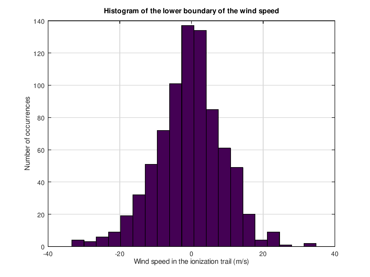
Which is consistent with the order of magnitude we expected for the mesospheric wind speed. One interesting thing about this histogram is that it is negatively skewed: it seems that fast negative speeds are slightly more common than fast positive speeds. I need additional experiments to confirm this trend, but this may suggest that off-line-of-sight reflections are slightly more frequent towards the east (as mesospheric winds blow from west to east in the winter hemisphere, see picture). This would make sense, as GRAVES transmitter is oriented towards the south, and France is at the east of Spain.

I will probably look into this in the near future. My next step is to repeat the experiment during the Leonids, which will peak around November 17th. I may get stronger signals and therefore better Doppler measurements.

Stay tuned!