
BatchDrake
Hacking, HAM Radio (EA1IYR), DSP, physics and more
Hacking, HAM Radio (EA1IYR), DSP, physics and more
In the previous post we managed to frequency-demodulate the video signal, putting the black level around 0. However, we concluded that since the baseband signal amplitude was unknown, it was impossible to universally map the luminance component to the right gray level: factors like signal bandwidth, sample rate or simply the baseband gain of the transmitter’s FM modulator will strongly affect the white and sync pulse level.
Before getting to the synchronization stage, we need to stabilize the signal amplitude in order to unambiguosly map each signal level to a given gray level. This operation is performed by the AGC block.
Software AGCs, as traditional analog AGCs, consist of a Variable Gain Amplifier (VGA) coupled to an amplitude detector and comparator. The detected signal amplitude at VGA’s output is used to compute an error signal that is used to dynamically adjust the VGA’s gain so the output signal’s amplitude is kept in the same level.
An VGA in C consists simply on the product of the signal by a some fixed gain value:
\[y[n] = Kx[n]\]Where \(K\) is the gain magnitude (and \(G=20log_{10}K\) the gain in dBs). The immediate amplitude of the signal can be calculated by:
\[a[n]=|y[n]|\]Of course, the immediate amplitude of the signal cannot be used directly to compute the error signal: the demodulated signal will oscillate between some more or less fixed levels, and we need to gather level information over enough time in order to produce a good amplitude estimation. A good staring point could be:
\[A[n]=\underset{0\leq i<m}{max}\left(a[n-i]\right)\]Which evaluates, at each sample \(n\), the greatest of the latest \(m\) samples. However, there are some limitations with this approach: if after \(m\) samples the maximum signal level drops quickly, the VGA’s gain will raise its amplitude identically fast, distorting the output signal and affecting the DSP chain performance afterwards. Also, what is the optimal value for \(m\)?
After the formula presented above, we can deduce that one key data structure of an AGC is some kind of sample array that keeps the last \(m\) samples. We will call this array the sample history. To prevent the AGC from constantly shifting the contents of its sample history (which is \(O(m)\) every time a new sample is added), it is a good practice to implement it as a circular buffer (in which addition is just \(O(1)\)).
The amount of time observed by the sample history can be easily related to its length by means of the sample frequency \(f_s\):
\[m=Tf_s\]If the maximum immediate amplitude is repeated with some periodicity \(T_A\), any \(m\geq T_Af_s\) will ensure that this maximum is always found in the sample history. For NTSC signals there are three periodicities to consider:
Of course, the longer the sample history is, the better the amplitude estimation will be, and we could be tempted to take the inverse of the vertical frequency as our sample history length. However, there are computational limits for this: if we capture video at a sample rate of \(f_s=20^6sps\), each field would spread along \(\frac{20^6}{59.94}\approx 334000\) samples. Every time a new sample is fed to the AGC, it would be compared against more than 300k samples in order to update its internal state. This is awfully slow.
Fortunately for us, it has been experimentally proven that taking the inverse of the horizontal frequency is enough to keep a good estimation of the signal amplitude, and therefore:
\[m_{good}=\frac{f_s}{15734 Hz}\]As we stated earlier, using the inverse of \(A[n]\) as the VGA’s gain is a bad idea, because transients may rise this estimation suddenly during \(m\) samples and then lower it back to a saner value. In general, this estimation is easily affected by noise.
One trick that works well in practice is to apply a single-pole IIR low pass filter on \(A[n]\), and use the result to compute a smooth-varying estimation of the signal level.
\(L[n] = (1 - \alpha)L[n-1] + \alpha A[n]\) As this level evolves smoothly, we can use it to calculate the VGA’s gain directly: \(K[n] = L^{-1}[n]\)
With \(\alpha\) being the only coefficient of the filter. The closer it is to 1, the faster it adapts to sudden changes of the signal level. Conversely, the closer it is to 0, the smoother the gain evolution will be.
Sigutil’s AGC is based on GQRX’s AGC and uses a slightly more sophisticated approach. Firstly, the immediate signal amplitude is expressed in dBFS and therefore:
\[A[n]=\underset{0\leq i<m}{max}\left(20log_{10}a[n-i]\right)\]Secondly, instead of keeping one amplitude level, it keeps two: the fast level and the slow level, being the \(\alpha\) of the first greater in general than that of the second. The final level estimation is taken as the maximum of both levels:
\[\begin{align} L_{F}[n] &= (1 - \alpha_F)L_F[n-1] + \alpha_F A[n] \\ L_{S}[n] &= (1 - \alpha_S)L_S[n-1] + \alpha_S A[n] \\ L[n]&=max(L_F[n], L_S[n]) \end{align}\]Which leads to: \(G[n] = -L[n]\)
since the signal amplitude level is expressed in dBFS. With this approach we get the best of both worlds: we can respond to transients quickly by rising the level estimation and lower it back as soon as it is over. However, the final estimation will not drop below the current slow estimation, which is in general closer to the true signal amplitude.
Thirdly, \(\alpha\) can be configured to have a different value if \(A[n]\) is greater or lesser than \(A[n-1]\). This makes sense, because a rise of the signal amplitude may mean that our previous estimate falls short and should be updated quickly. However, a fall of the esimated amplitude may simply mean that the signal is changing its sign, and it is not as significant as a rise.
In many practical applications, the signal of interest may become silent for a while before continuing. This is especially true in NTSC: if the transmitted image goes suddenly dark, the AGC should wait some time before updating the amplitude estimation. This amount of time is called the hang time.
In Sigutils, the hang time is used for slow level updates, but not for fast level updates. The rationale behind this is that the fast level update is used to neutralize short transients, and in general it is not meant to be used as a true amplitude estimator.
The coefficient \(\beta=1-\alpha\) of the aforementioned low pass filter is also known as the decay factor. This filter is a recursive filter, and therefore its impulse response must be infinite. In fact, the analytic expression of its impulse response looks like this:
\[h_\alpha[n]=\begin{cases} \alpha\beta^n & n \geq 0 \\ 0 & n \ < 0 \end{cases}\]It is common to express \(\alpha\) and \(\beta\) in terms of the time constant \(\tau\):
\[\begin{align} \beta &= e^{-\frac{1}{\tau}} & \alpha &= 1 - e^{-\frac{1}{\tau}} \end{align}\]Which represents the numer of samples it takes for the output to decrease to 38.6% of the original value. Since this value is more intuitive than a dimensionless number between 0 and 1, and it can be unambiguously related to the filter behavior in sample units, it was the final choice for the AGC configuration structure.
 for the single pole low pass filter. In red: 38.6% of the value at \\(h[0]\\).")
The last quirk of sigutil’s AGC is the presence of a delay line, which is implemented as another circular buffer that keeps the last \(d\) samples fed to the AGC. Since the amplitude levels take some time to stabilize before they become useful (especially during a transient), the AGC’s output is delayed as well so that the amplitude level estimation can be applied to the samples that modified it in the first place.
Finally, the computed signal amplitude level is used to adjust the gain of the VGA and return a digital signal of constant amplitude 0.5 (1 peak-to-peak).
Having all this in mind, here are some quantities that will work well for a NTSC signal. Note that although some of these values were theoretically deduced, most of them were experimentally found:
Now we are ready to stabilize the demodulated signal’s amplitude through Sigutil’s AGC (defined in <sigutils/agc.h>). AGC configuration is done through struct sigutils_agc_params, which sould be initialized with sigutils_agc_params_INITIALIZER. The magic numbers above would lead us to the following code:
struct su_agc_params agc_params = su_agc_params_INITIALIZER;
su_agc_t agc;

agc_params.mag_history_size = SAMP_RATE / 15734.0;

agc_params.delay_line_size  =  agc_params.mag_history_size;
agc_params.fast_rise_t = 0.2 * agc_params.mag_history_size;
agc_params.fast_fall_t = 0.5 * agc_params.mag_history_size;
agc_params.slow_rise_t = 1.0 * agc_params.mag_history_size;
agc_params.slow_fall_t = 1.0 * agc_params.mag_history_size;
agc_params.hang_max    = 525 * agc_params.mag_history_size;

if (!su_agc_init(&agc, &agc_params)) {
  fprintf(stderr, "error: failed to initialize AGC\n");
  exit(EXIT_FAILURE);
}
And the processing loop will now look like this:
  prev = 0;
  while (fread(&x, sizeof(SUCOMPLEX), 1, fp) == 1) {
    x *= su_ncqo_read(&nco1);      /* Center spectrum */
    x = su_iir_filt_feed(&lpf, x); /* Filter centered signal */
    x *= su_ncqo_read(&nco2);      /* Center signal around the black level peak */
    y = carg(x * conj(prev));      /* Perform FM detection */
    prev = x;                      /* Save previous sample */
    y = su_agc_feed(&agc, y);      /* Stabilize amplitude */
    fwrite(&y, sizeof(SUCOMPLEX), 1, ofp);
    ++samples;
  }
The full code can be downloaded here.
The processing of the signal is now many times slower because of the math carried out by the AGC. This is expected, and the AGC is probably one of the slowest blocks inside Sigutils. If we open the file with Audacious, we should see something like this:
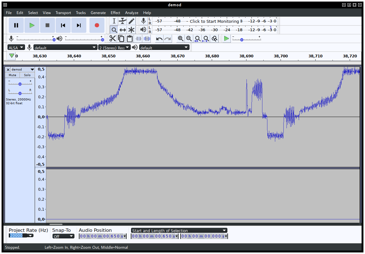
Which is the constant amplitude signal (0.5 or 1 pk-pk) we were looking for.
Now, the NTSC baseband signal is ready for video processing. In the next article we will see how to find the horizontal sync pulses and use this information to extract the first captures of the transmitted pictures.
Stay tuned!