GRAVES, SigDigger and direction finding (II)

This is the second part of a series about radio direction finding. Read the first post on the series here

The constraints

It was already mid-summer, July was approaching to its end, and the amount of time I had to implement this direction finding feature for SigDigger was limited. Perseids have their peak activity at around August 12th, and SigDigger (or more precisely, Suscan) suffered from a big shortcoming: it was not designed for MIMO use cases.

In short, SigDigger is mostly a GUI for Suscan, and Suscan treats signal sources as a stream of complex I/Q samples received from somewhere. These samples are delivered to SigDigger at certain sample rate, and are assumed to come from a single RF input. This means that I have only one spectrum every time, and all the inspectors I open are fed by that spectrum alone.

Unfortunately, this use case requires reading samples from both inputs (RX1 and RX2) at the same time, and performing continuous phase comparisons between both. I had two options:

• I refactor Suscan completely, so that sources can now provide more than one sample stream at the same time. This impacts how spectrums should be treated and represented, how FFTs are scheduled among workers, how inspectors are fed, and what kind of UI I present to the user, or
• I write an ugly kludge that multiplexes both channels in frequency, and treat RX1 and RX2 as two channels with different frequencies.

August had already begun, so I settled for the latter. I am sorry.

The kludge

The AntSDR plugin provides two different things: a graphical, phase comparison tool certain (namely, “Phase Comparator”) and the implementation of a “2RX combined signal source”, selectable from SigDigger’s settings dialog. This signal source bypasses the single-input limitation by performing the following trick:

1. Adjusts the AntSDR radio bandwidth to something relatively small (i.e. well below 1/8th of the sample rate)
2. Takes the samples from RX1 and performs a downwards frequency shift of 1/4 of the sample rate to them
3. Takes the samples from RX2 and performs an upwards frequency shift of 1/4 of the sample rate to them
4. Sums both and delivers the result back to SigDigger.

As a result, the signal source fits the spectra of the two inputs in a single input spectrum by multiplexing both in the frequency domain. Additionally, the multiplexing is performed so that a fixed phase relationship between both channels is ensured. This enables reliable phase comparisons between the inputs by exploiting the existing channel inspection abstraction provided by Suscan: it boils down to opening raw inspectors on the frequency-shifted inputs and comparing the samples of both.

Into the guts of phase comparison

There are a few ways to perform phase comparisons between both antennas. The one I chose for the Phase Comparator is based on the following discrete signal, synthesized from the samples of both antennas:

\[y[n]=x_1[n]\bar{x}_2[n]\]

Where \(x_1[n]\) the samples from RX1 and \(x_2[n]\) the samples from RX2. The comparator signal \(y[n]\) has an amplitude that is proportional to the product of the amplitudes of both inputs, and a phase that equals that of the difference between both. The upper bar on \(x_2\) indicates that the samples of the second antenna must be conjugated, i.e. the sign of its imaginary component flipped.

The math behind this is not too complicated. Since the samples of any antenna \(x[n]\) can be expressed in polar form as the product of an absolute value \(A[n]\) and a complex phase term of \(\phi[n]\) radians:

\[x[n]=A[n]e^{j\phi[n]}\]

the conjugation operation (which is computationally cheap, as it reduces to flipping a sign bit) results in an inversion of the sign of the phase, and therefore:

\[y[n]=x_1[n]\bar{x}_2[n]=A_1[n]e^{j\phi_1[n]}A_2[n]e^{-j\phi_2[n]}\]

from which follows that:

\[y[n]=A_1[n]A_2[n]e^{j\Delta\phi[n]}\]

with \(\Delta\phi[n]\) being just the argument of \(y[n]\). This signal is directly represented in the plugin’s Phase Comparison tab as a colored wave envelope, with each color representing a different phase difference.

Event logging

One of the fancy things provided by the AntSDR plugin is to perform automatic event detection, a feature similar to that provided by clistones. While clistones relies on an SNR criterion to detect events, the plugin leverages the extra information provided by both antennas to perform a more sophisticated guess, which works as follows: we start by stating that we expect echoes to be point-like, i.e. to maintain the same phase difference along their timespan. This imples that the absolute value of the phase of the following complex quantity:

\[z[n]=y[n]\bar{y}[n-1]=A_y[n]A_y[n-1]e^{j(\Delta\phi[n]-\Delta\phi[n-1])}\]

should be small, as \(\phi[n]\) is expected to be not too different from \(\phi[n-1]\). Conversely, in the presence of noise alone, the phases of two consecutive complex samples would follow a uniform random distribution between \(-180º\) and \(180º\). In case you were already wondering, yes, this is just an FM quadrature demodulator applied to the phase comparator output. In this case, the silence at the output of the FM demodulator can be used to signal the presence of an event.

I relied on a smoothed measurement of the square of the phase of \(z[n]\) to generate the detector signal \(D[n]\). This smoothed measurement is just the output of a single-pole low-pass filter with time constant $\tau/f_s$, with \(\tau\) the smallest duration of the events we expect to find and \(f_s\) the sample rate of the channel. From this, it follows that the only tap of the filter is given by \(\beta=1-e^{-f_s/\tau}\), and \(D[n]\) is evaluated as:

\[D[n]=\beta\text{arg}(z[n])^2+(\beta-1)D[n-1]\]

The square root of \(D[n]\) is then compared against certain threshold angle \(\varphi_e\) provided by the user. If \(D[n]\) falls below \(\varphi_e\), an event is considered to have started. On the other hand, if \(D[n]\) stays above this threshold for some time (called the hold period) after the start of the event, the event is considered to have finished.

This, of course, begs the question: how do we choose an appropriate threshold? We said earlier that, in the presence of noise, \(\text{arg}(z[n])\) follows a uniform distribution. However, this is no longer true for \(\text{arg}(z[n])^2\) (give a look to this post in StackExchange for details). In fact, \(\mathbb E[\text{arg}(z[n])] = 0º\) but \(\sqrt{\mathbb E[\text{arg}(z[n])^2]}\approx 103.9º\). This value is our noise ceiling: \(\varphi_e\) must be necessarily smaller than this. As we lower \(\varphi_e\) closer to 0º we make the detection algorithm less and less sensitive, and only the events with the highest degree of phase coherence will be detected.

These two parameters (\(\tau\) and \(\varphi_c\)) could be adjusted from Event Logger’s tab of the AntSDR plugin. In my case, I wanted to detect very faint events, so I set the threshold to \(80º\). On the other hand, to reduce the number of false positives caused by random fluctuations (\(80º\) is very close to the noise ceiling) I set \(\tau\) to 100 ms.

The plugin

The AntSDR plugin in action, highlighting some events

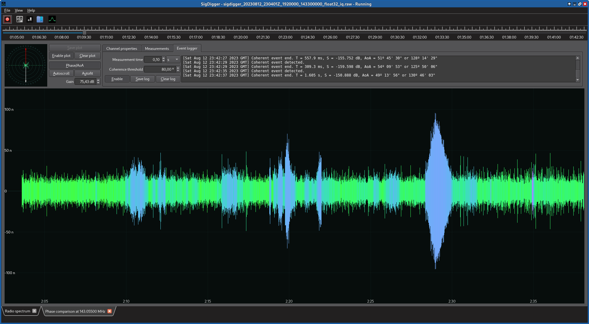
The plugin was made minimally functional right before the deployment of the antenna, although it not was completed until some time after. It features a phase / AoA view in the top-left corner of the phase comparison tab, and plots the phase comparator output (our \(y[n]\)) on a SuWidget’s Waveform widget. The Waveform widget was configured to display only the evelope of the signal, colorizing it with the instantaneous phase of each sample.

The plugin also enables manual adjustment of certain parameters (detector parameters, dipole separation, maximum buffer size, etc), phase and angle measurements, data saving and event logging.

The night of the observation

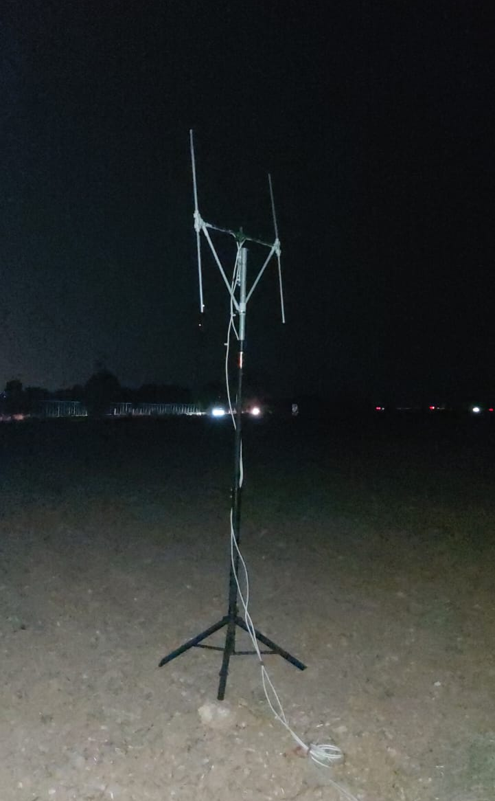
I leveraged the opportunity to gather with some friends and do some stargazing. Array, receiver, laptop, SigDigger and a telescope (definitely a must) were all deployed on the night of August 12th 2023 in Cerro del Viso, near Alcalá de Henares (Spain).

Unsurprisingly, the deployment was harder than predicted. First, it was so dark that I did not have many references to have a perfect alignment to the North, so I had to eyeball it towards the Pole Star. Next, after connecting everything, I realized the cables were flipped and hence the reference direction was pointing South. Not a big deal (can be fixed in a post-processing phase), but it was something I had to remember. The array plane was also tilted, firstly because of the irregular terrain, and second due to my lame attempts to correct these irregularities by moving the tripod here and there. And of course, my favourite one: the hard disk I took with me to save the raw IQ data was so slow it swamped SigDigger all the time, so I had to save the recording directly to my laptop.

The antenna array, deployed the best I could

Despite the obstacles, a successful recording of 36.1 GiB was produced, containing more than 30 minutes of raw IQ data. I made a backup of the file to my external (and slow) hard drive, which was later uploaded to Zenodo (download the full 36.1 GiB capture file here).

In parallel with the data capture, the AntSDR plugin was kept running to have visual feedback on the events being recorded. Additionaly, the audio inspector was set to SSB and opened 1 kHz apart from the GRAVES central frequency, thus providing audible feedback of the events (the pings we all know and love).

Data reduction

The capture file was analyzed a few days later with SigDigger, and the event logger was adjusted to the parameter values described earlier. A total of 42 strong events were detected and saved to a CSV file directly from the AntSDR Plugin’s Event Logger GUI (download it here).

Each line of the CSV file corresponds to a detected event, and has the format:

ts_s,ts_u,phase,rms,angle1,angle2,power,duration

Where:

• ts_s and ts_u: timestamp of the beginning of the event, according to the source time. ts_s is seconds since the Unix epoch, and ts_u is the number of microseconds that have to be added to ts_s
• phase: mean phase of the detected event
• rms: RMS of the detector signal (currently a placeholder, fixed to 0)
• angle1 and angle2: possible angles of arrival
• power: Mean power of the event, in dBs of arbitrary units
• duration: Duration of the event, in seconds

The CSV file was processed using this Jupyter lab notebook (HTML), and the possible angular solutions to the detected events represented by means of a polar plot. In this plot, the solutions that fall in front of the array are painted in blue, while the solutions behind the array are painted in orange. The dashed line represents the dipole array plane. The radial distance of the events is proportial to their mean power, and their are is proportional to their duration.

Results

Two representations were produced: one containing all possible angular solutions, and another one removing the SE / NW quadrants.

Polar representation of the plugin's event log. Angle solutions in the forward direction (North) are painted in blue. Solutions in the backward direction (South) are painted in orange. The plot in the right removes SE and NW quadrants to highligh the event alignment.

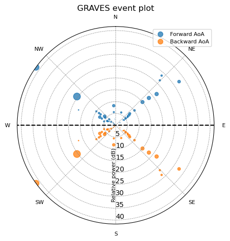
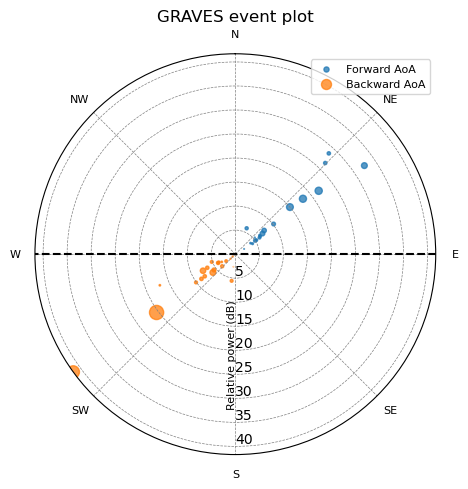
From the plot in the right, it is clear that most events fall into a straight line of roughly 53º from North to East. Representing this line on a map, we can see that it falls between the RX and TX site, being somewhat closer to the RX than the TX. This seemed consistent with observations by previous researchers.

The 53º line-of-sight.

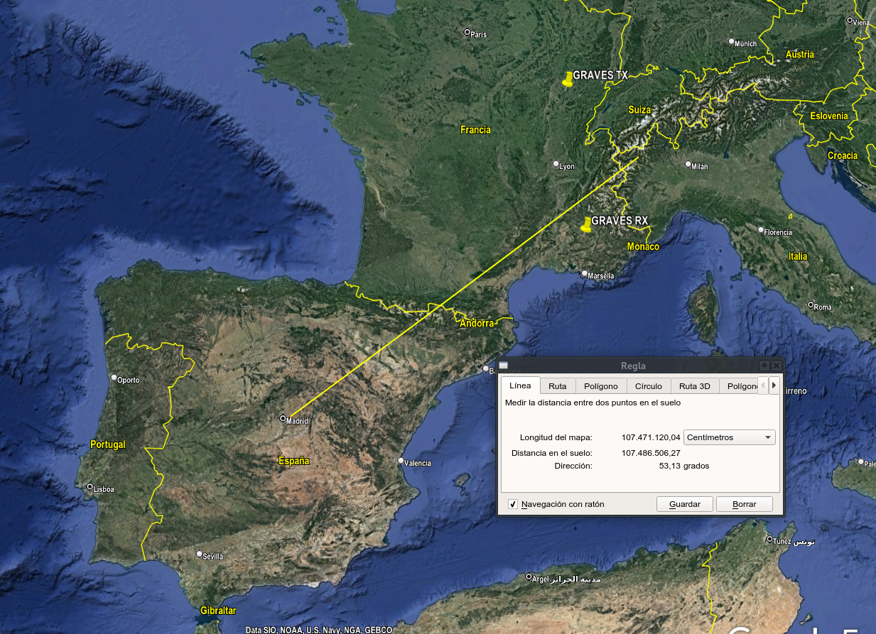
The NE events seem easy to explain: the radar’s beam has an elevation of \(\text{El}=25 \pm 10º\) and it is oriented towards the South of France. Measured with Google Earth, the point in which the 53º line crosses the TX-RX line of sight is 262 km apart from the TX site. Since this distance is small compared to the radius of the Earth, we can approximate the height at which the beam passes by \(h = 262º \text{tan}(\text{El})\). From this we can conclude that, at that point, the beam passes \(145 ± 80\text{ km}\) above the ground (which already overlaps the mesosphere, located between \(50\text{ km} - 85\text{ km}\)). And this is not even its closest point to TX in the observed direction.

More difficult to explain are the SW events (NW?) events. Miguel EA4EOZ suggests these may be back-scatter events, but the beam should be passing more than $600 \pm 300\text{ km}$ above Madrid, with increasing distance as we move SW. While I could not find any explanation that convinced me, I came up with a list of possibilities worth exploring:

• The alignment of the antenna is just wrong, and the beam is actually wider than described. Only events aligned with the TX can be heard, and these events are truly backscatter.
• Excess total electron content in the ionosphere due to the trail, causing reflection at very high altitudes.
• The beam got reflected due to grazing incidence on the lower layers of the ionosphere?
• Or Miguel’s all-time favorite hypothesis: perhaps something occurring at a few meters from the receiver?

This is an open question to me, and other possible explanations I did not think of are welcome!

Conclusions

The experiment was fun, although a bit frustrating at times. It provided me with results that make sense (confirming that my antenna is not rubbish) and with results I cannot explain (which invites me to repeat the experiment at some point in the future). But the bottomline is clear to me: I finally managed to get coherent samples out of the AntSDR, and more experiments with coherence will happen in the future. And yeah, Suscan should support coherent channels at some point.

Stay tuned!